Environmental Engineering Reference
In-Depth Information
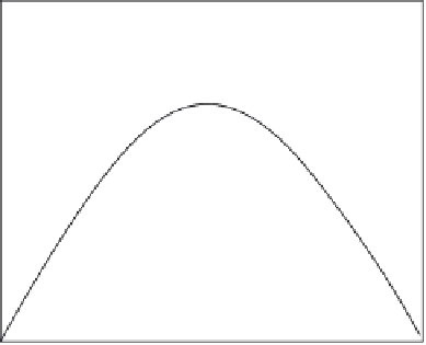
Figure 18.4 illustrates a typical EKC curve with income per capita on the
X
-axis and envi-
ronmental degradation, i.e., pollution, on the
Y
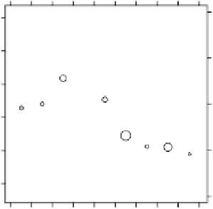
-axis. Figure 18.5 illustrates the real EKC for
arsenic pollution in water of a river basin.
A great deal of research and investigation have been carried out after Grossman and
Krueger's work (Bruvoll and Medin, 2003; Jha and Murthy, 2003; Cole, 2004; Paudel et al.,
2005; Paudel and Schafer, 2009; Jordan, 2010; Culas, 2012) to examine the accuracy of the EKC
for various environmental degradation indicators such as air pollution (Bruvoll and Medin,
2003; Cole, 2004), water contaminants (Paudel et al., 2005; Paudel and Schafer, 2009), and defor-
estation (Culas, 2012). While much research was consistent with the EKC theory (Munasinghe
and Swart, 2004; Culas, 2012; Munasinghe, 1999; Hwang, 2007) and shows a bell-shaped trend
through the per capita income changes, there are some investigations that are incompatible
with the EKC theory (Grossman and Krueger, 1995; Culas, 2012). Figure 18.6 shows a compari-
son for a number of published articles relevant to the EKC that were conirmed and rejected.
Tu rning point income
Environmental
decay
Environmental
improvement
Per capita income
FIGURE 18.4
EKC proposed by Grossman and Krueger. (From Grossman, G.M., Krueger, A.B.,
J. Econ.
, 110, 353, 1995.)
GEMS/WATER: arsenic in rivers
3
.02
.015
2
.01
1
.005
0
0
-.005
-1
0246810
GDP per capita (1985 $1000s)
12
14
16
18
FIGURE 18.5
Relationship between per capita GDP and heavy metals contamination of rivers. (From Grossman, G.M.,
Krueger, A.B.,
J. Econ.
, 110, 353, 1995.)