Image Processing Reference
In-Depth Information
1
λ
R
1
(
−
)
=
, is the same as that in
Eq. (
4.6
). Hence, the maximum achievable savings factor in this case is also the same,
i.e.
Corollary 2
:FromEq.(
4.10
), max
r
k
ln
1
−
κ
1
S
=
.ButEq.(
4.10
) does not tell us how tight is the bound.
λ
R
ln
(
1
−
κ)
1
−
Corollary 3
:If
H
(
I
r
)
is high, it can tolerate a proportionally larger perturbation
Δ
.
4.4 Experimental Results
We shall substantiate the effectiveness of the band selection scheme over the two
datasets- the urban data, and the moffett
2
data. We shall demonstrate the results using
the bilateral filtering-based fusion technique discussed in Chap.
3
as the readers are
conversant with the same.
The results show that in both datasets the fused images over the subsets of both of
the test data, selected using the conditional entropy-based technique are comparable
in quality to the resultant images generated over the fusion of entire dataset using
the same fusion technique.
Since the available bands in hyperspectral data are ordered according to wave-
length, we can employ the specific case of the entropy-based selection scheme,
and select the bands using Eq. (
4.4
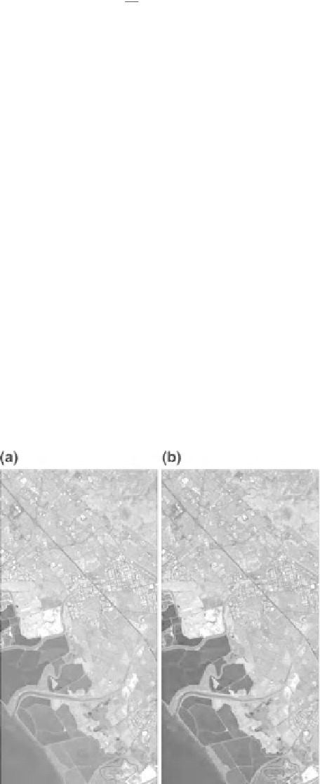
). Figure
4.2
a shows the result of fusion for the
Hyperion data using the bilateral filtering-based fusion technique where only 27
selected image bands have been fused. This figure may be compared to Fig.
4.2
b
which represents the fusion of the entire hyperspectral data cube. It can be seen
Fig. 4.2
Results of fusion
of the Hyperion data applied
over a subset of bands selected
using the conditional entropy-
based approach.
was set to
0.50 and only 27 bands were
selected.
a
shows the results
of bilateral filtering-based
fusion over the selected bands.
b
shows the corresponding
result of fusion of the entire
data (© ACM 2010, Ref: [87])
κ


