Image Processing Reference
In-Depth Information
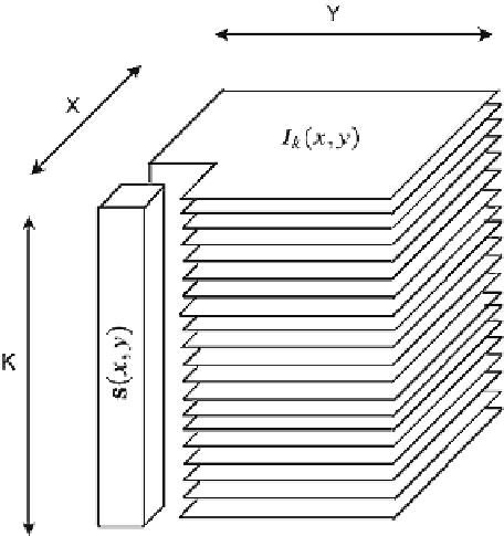
Fig. 2.3
Illustration of the
notations for a hyperspectral
image
This image can be considered as a set of
K
two-dimensional spectral bands. We
shall denote the
k
-th band by
I
k
,
K
. Each
I
k
, therefore, refers to a 2-D
spatial plane. The gray value of the pixel at the location (
x
k
=
1
,
2
,...,
,
y
) in this band is given
by
I
k
(
.
The hyperspectral image
I
contains spectral signatures of the pixels covered by the
spatial extent of the imaging sensor. The image, therefore, is a collection of spectral
signatures across locations
x
,
y
)
(
x
,
y
),
x
=
1
,
2
,...,
X
;
y
=
1
,
2
,...,
Y
. Each of the
spectral signature is a vector of dimensions
. A pixel in the fused image is
primarily generated by processing the spectral signature of the pixel that represents
an array of observations across all spectral bands for the given spatial location.
We shall often work with this 1-D spectral array at a given location. Therefore,
we shall introduce a different notation to refer to the spectral arrays (or vectors)
in the hyperspectral image
I
. We shall denote the array of observations (i.e., the
spectral signature) at location
(
K
×
1
)
. It may be noted that this
notational change is purely meant for the ease of understanding as the same data will
be referred from different dimensions. Figure
2.3
illustrates the relationship between
the two aforementioned notations. A hyperspectral image
I
, thus, can be considered
as a set of bands
I
k
where the set contains
K
elements. The same image can also be
considered to be a set of spectral arrays
s
(
x
,
y
)
by
s
(
x
,
y
)
∀
(
x
,
y
)
(
x
,
y
)
where the set contains
XY
elements.