Java Reference
In-Depth Information
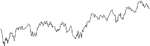
DJ INDU AVERAGE (DOW JONES & CO)
as of 11-Apr-2006
11500
11000
10500
10000
May05
Jul05
Sep05
Nov05
Jan06
Mar06
Figure 18-3
Dow Jones Industrial Average time series data (graph courtesy
Yahoo! Finance).
These patterns are often characterized as
trend, cycle,
and
irregular
components—referred to as the
decomposition
of the time series. The
trend reflects the long-term change in the average value of the time
series signal. Here, long term depends on the sampling rate of the
time series signal. The cycle reflects any repeating pattern of the sig-
nal, which can be characterized into
seasonality
or
periodicity
. If the
cycle is seasonal, effects occur at specific times (e.g., “every Thanks-
giving,” “every quarter,” or “every Friday”). If the cycle is periodic,
the cycle repeats itself every
n
time periods. Cycles, in general, are
described in terms of both a
period
and a
resolution
.
As with all data mining, the model produced from the data is
imperfect. Not all the variation in the data can be expressed in regu-
lar trends or cycles. This residual difference, what is left over after
removing everything that can be explained from the series, is
referred to as the irregular component. Figure 18-4 illustrates the
decomposition of a time series into its seasonality and trend with
residual or irregular component.
As discussed earlier, time series analysis can help to show the
structure or patterns found in the time series data, but it can also be
used to forecast signal values in the future (e.g., forecasting the stock
market and other economic indicators, retail product demand, and
even weather predictions). Forecasts can be short range, such as the
next period or few periods (which often maps to hours or days), but
can also be long range, projecting results months or years ahead.
Figure 18-5 illustrates a forecast for the time series data example.
Since forecasts, or predictions, are in one sense statistical estimates,


Search WWH ::

Custom Search