Environmental Engineering Reference
In-Depth Information
σ
v
σ
v
P
P
σ
h
τ
f
σ
h
(4) Passive state
of failure
σ
f
τ
f
σ
f
(3) Active state
of failure
(2) After slight
movement
(1) At rest
(1) At rest
(3) After more
movement
(2) After
movement
σ
h
1
σ
h
2
σ
v
=
σ
h
σ
h
3
σ
h
4
σ
h
3
=
K
p
σ
v
=
K
a
σ
v
σ
h
2
σ
3
=
σ
h
1
σ
1
=
σ
v
Q
Q
45 +
/2 to
plane
on which
σ
1
=
Slip lines
45 +
Slip lines
/2 to plane
on which
σ
1
=
σ
h
acts
σ
h
acts
Compression
Extension
(a)
(b)
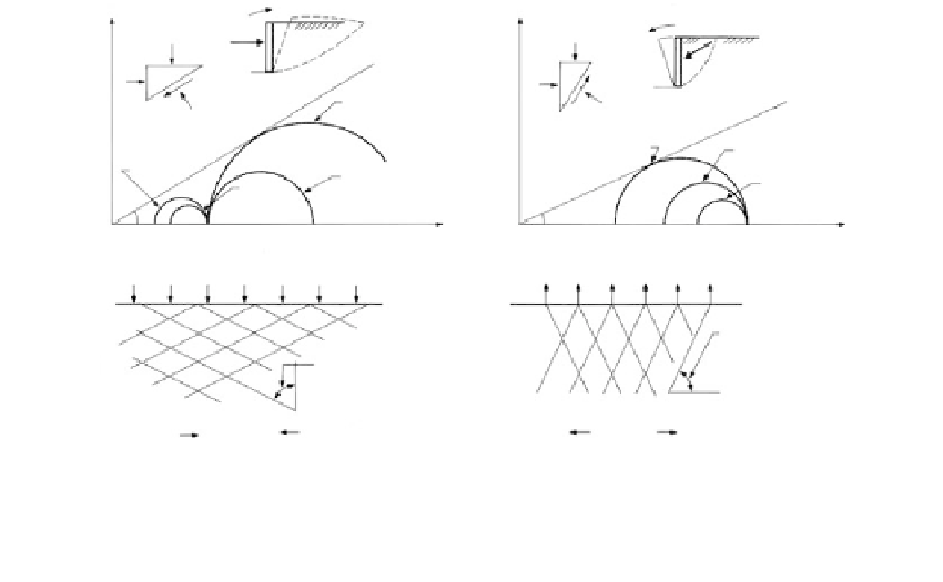
FIGURE 3.35
Mohr diagrams for the (a) passive and (b) active states of stress.
or
σ
v/
σ
h
tan
2
(45
°
φ
/2)
K
p
(3.37)
where
K
p
is the coefficient of passive stress.
Active State of Stress
The active state exists when a soil mass is allowed to stretch, for example, when a retain-
ing wall tilts and
σ
v
remains unchanged and
σ
h
decreases (2) until the induced shear stress is sufficient to cause failure (3). At this point
of plastic equilibrium, the active state has been reached.
The coefficient of active stress
K
a
, (the ratio
σ
v
σ
h
. In Figure 3.35b, as the mass stretches,
σ
v
) represents a minimum force,
expressed for a cohesionless soil with a horizontal ground surface as
σ
h
/
K
a
tan
2
(45
°
φ
/2)
(3.38)
and
K
a
1/
K
p
(3.39)
Applications
The
at-rest coefficient K
0
has a number of practical applications. It is used to compute lateral
thrusts against earth-retaining structures, where lateral movement is anticipated to be too
small to mobilize
K
a
. It is fundamental to the reconsolidation of triaxial test specimens
according to an anisotropic stress path resembling that which occurred
in situ
(CK
o
U tests).
It is basic to the computation of settlements in certain situations (Lambe, 1964). It has been
used for the analysis of progressive failure in clay slopes (Lo and Lee, 1973), the prediction
of pore-water pressure in earth dams (Pells, 1973), and the computation of lateral swelling
pressures against friction piles in expansive soils (Kassif and Baker, 1969).