Environmental Engineering Reference
In-Depth Information
3
1.6
1.4
1.2
2
1.00
0.80
0.60
1.0
0.40
0.20
0
0
0
2.0
4.0
6.0
8.0
10.0
0
1.0
2
3
Time
4
5
6
Time
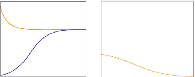
Fig. 6.4
Left
: Temporal dynamics of (6.9) (initial condition:
N ¼
1.5 for the
upper curve
and
N ¼
0.05 for the
lower one
). The stable equilibrium is at
N
¼
1.0.
Right
: Temporal dynamics of (6.10)
(initial condition:
N
¼
1.0015 for the upper curve and
N
¼
0.95 for the lower one). The unstable
equilibrium is at
N
¼
1.0
At all intermediate steps, model behaviour is tested to make sure that even in
complex situations the overview does not get lost. This approach is called rapid
prototyping and is frequently applied in various modelling approaches. The Lotka-
Volterra equations can be considered as a simple prototype of a predator-prey
system. The equations are:
dPrey
dt
¼
C
1
Prey
C
2
Prey
Pred
(6.11)
dPred
dt
¼
C
2
b
Prey
Pred
C
3
Pred
To understand the model, we first look at the different components of the
equations.
Prey
represents the size of the prey population.
Pred
represents the size of the predator population.
In the literature, predator and prey are frequently denoted as
N
1 and
N
2, which
we will use also below.
dPrey
=
dt
represents the extent of change in the prey population at each point in
time.
dPred
dt
represents the extent of change in the predator (pred) population at
each point in time.
=
-
C
1,
C
2,
C
3 and
b
are positive constants. In typical cases, they have a small value
below 1.0.
-
C
1 is the rate of increase per unit of time (growth rate) for the prey population.
-
C
2 is a predation factor, specifying what fraction of prey will be caught per unit
of time depending on the size of the predator and prey population.