Environmental Engineering Reference
In-Depth Information
MD Piedmont Forests
1.0
0.8
0.6
0.4
LC 1999
MX 1999
0.2
0.0
-2
0
2 4
In(Patch Size)
6
8
10
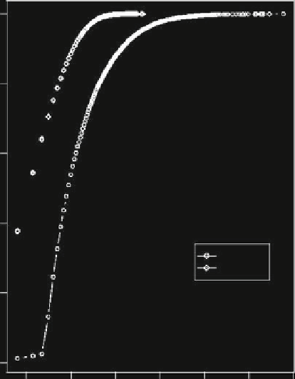
Fig. 15.1 The cumulative frequency distribution of forest patches within the Maryland Piedmont
(
open circles
) in 1999 contrasted with the cumulative frequency distribution of random patches
(
open diamonds
) generated by the RwC method using Qrule (see text for details)
model generated random patterns within the restricted area defined by the 1992 land
cover map (i.e. its selected boundaries shown in Fig.
15.2
plus lakes and rivers).
Under some circumstances the map constraints may be sufficient to cause the RwC
model to produce patterns that differ substantially from a random map without
constraints (see discussion of the association matrix below). Because the restric-
tions of the Maryland Piedmont map are not severe (Fig.
15.2
), the general patterns
are similar to those of a simple random map (cf. Gardner et al. 1987; Gardner and
O'Neill 1990; Zar 1996) (Fig.
15.2
).
The statistical differences among landscape metrics can be graphically illustrated
with box and whisker diagrams. Figure
15.3
plots the distribution of Sav for forested
and urban areas, contrasting the distributions of values from the RwC simulations for
1992 and 2001. The values for the actual landscapes are beyond the range of the RwC
generated values (Table
15.2
) and are not plotted here. Figure
15.3
shows that the
range of values for Sav from the RwC simulations were very small (C.V.
1%) with
clearly different values for 1992 and 2001. Because patterns generated by the RwC
model are due to random processes, this difference is entirely due to the shifts in
p
for
<