Environmental Engineering Reference
In-Depth Information
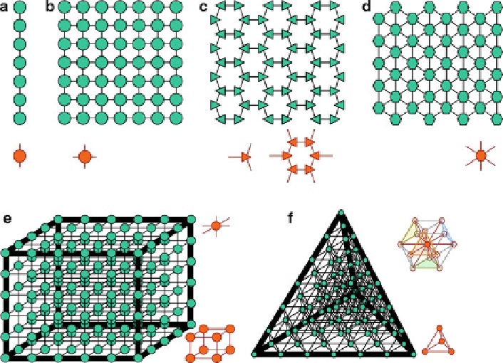
Fig. 8.1 Examples of one-, two- and three-dimensional grids of different topologies. (a) Linear
grid: each cell has two neighbours; (b) 2D rectangular grid: each cell has four neighbours; (c)2D
triangular grid: each cell is connected to three neighbours; (d) 2D hexagonal grid: each cell has six
neighbours; (e) 3D cubic grid: each cell inside the grid has six neighbours; (f) 3D tetrahedral grid:
A cubic grid is not the only possibility to model in three dimensions. An alternative could consist
of cells connected at the edges of stapled tetrahedrons. Please keep in mind that the given
neighbourhood relations do not apply for margin cells
The Neighbourhood
The neighbourhood comprises the cells in the surrounding of a focal cell. The
neighbourhood cells are defined as those that can influence the state of the
particular focal cell. To determine which change occurs, the state of the focal
cell and the states of the neighbourhood cells are evaluated. Usually, the neigh-
bourhood consists of the directly adjacent cells, but the neighbourhood can have
different extents and can vary in shape between rectangular, circular, etc. Other
definitions are possible as well, e.g. that each cell selects a random number of
other cells as neighbours - regardless where they are located on the grid. In case
of a rectangular two-dimensional grid (Fig.
8.1b
), the most commonly used
neighbourhood comprises the four direct neighbours (Fig.
8.2b
). In the CA
terminology, this is also called von Neumann neighbourhood. If the eight directly
adjacent cells are considered as neighbours, it is called Moore neighbourhood
(see Fig.
8.2c
), named after the US-American mathematician Edward F. Moore
(1925-2003).