Environmental Engineering Reference
In-Depth Information
5
5
0
5
0
5
x
x
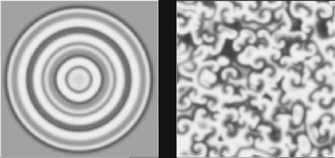
Fig. 7.5 Generation of target patterns and spiral waves of (
7.10
and
7.11
). Parameters:
r ¼
K ¼
1,
a ¼ b ¼
10/3,
e ¼
2,
m ¼
4/5,
g ¼ h ¼ Y
3
¼
0,
D
1
¼ D
2
¼
1 (a.u.), no-flux boundary
conditions
7.4.3 Diffusion-Induced Chaos in Heterogeneous Environments
So far we have assumed that the environmental conditions relevant for species
growth and interaction do not explicitly depend on the spatial position, i.e. the
parameters are constant all over the spatial domain. However, it was already
implied in (
7.2
), that the growth term
f
may explicitly depend on the spatial
location
x
. This allows one to incorporate heterogeneous environmental conditions
into the spatial model. One effect of a heterogeneous environment in a spatially
one-dimensional variant of model (
7.10
and
7.11
) has been presented by Pascual
(1993), assuming a linear increase in the prey growth rate
r
(
x
)
cx
. Assum-
ing that the system is in the oscillatory regime at all spatial locations, this leads
to a line of infinite diffusively coupled non-identical oscillators. Following the
temporal change of population density Y(
t
) at fixed spatial locations
x
indicates
that the local dynamics undergo a transition from regular oscillations at high prey
growth rate to quasi periodic and finally chaotic oscillations at low prey growth rate.
This is shown in Fig.
7.6
.
¼
r
0
þ
7.5 Concluding Remarks
The examples given above can be generalized to
N
interacting species in three
dimensional space, which are subject to diffusive and advective motion and envi-
ronmental fluctuations. This leads to the following equation for the rate of change
for the
i
th species: