Environmental Engineering Reference
In-Depth Information
dN
1
dt
¼
N
1
r
1
ð
a
11
N
1
a
12
N
2
c
1
N
3
Þ
(6.19)
dN
2
dt
¼
N
2
r
2
ð
a
21
N
1
a
22
N
2
c
2
N
3
Þ
dN
3
dt
¼
N
3
bc
1
ð
ð
N
1
þ
c
2
N
2
Þ
d
Þ
with
r
1
¼
1;
r
2
¼
1;
a
11
¼
0.001;
a
12
¼
0.001;
a
21
¼
0.0015;
a
22
¼
0.001;
c
1
50.
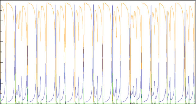
The Gilpin equations (6.19) describe a predator population (
N
3) and two com-
peting prey populations (
N
1,
N
2). The only new aspect to what we have discussed
so far is the inclusion of competition. It relates to logistic growth, in which growth
of a population is limited to a finite total carrying capacity, where the increase of
each competing population is limited by both its own size, and the size of the
competing population, in terms of a competition coefficient. Without predators, in
Gilpin's model one prey population would be outcompeted and go extinct. Both
populations persist through the predator's influence, which modulates the competi-
tion effect. This model was used as a default for the “interaction engine”, a simple
differential equations integrator of the POPULUS software (Alstad 2007). Fig-
ure
6.10
shows the simulation of the three variables over time. In Fig.
6.11
it
looks “as if ” the trajectories would cross, but this is only because a projection of
only two of the three variables in a plane was shown (
N
2 over
N
1). There are also
other ways in which deterministic chaos can occur in the interaction of three
¼
0.01;
c
2
¼
0.001;
b
¼
0.5;
d
¼
1 and the initial conditions
N
1
¼
N
2
¼
N
3
¼
1000
800
600
400
200
0
0
1000
2000
Time
Fig. 6.10 Gilpin's Spiral Chaos Attractor. The simulation results of (6.19) with the initial
conditions
N
1
¼
N
2
¼
N
3
¼
50
.N
1
,N
2 and
N
3 are plotted over time (3,000 time steps)