Basics of Environmental Sampling and Analysis - Fundamentals of Environmental Sampling and Analysis - page 22

log-normal distribution. Mathematically, the normal distribution can be described as
the following function:

2

ðÞ

e 2

x m
s

y ¼

s

p ð1 < xþ1Þ ð2 : 18Þ

2p

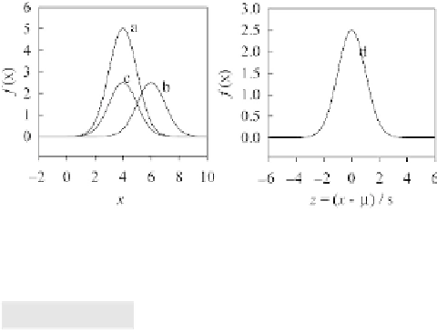
This function can be defined by two parameters, the mean (m) and the standard
deviation (s). Figure 2.3 shows the normal distribution of three different data sets (a,
b, and c) and a normalized ''standard normal distribution'' (d). The standard normal
distribution is similar in shape to the normal distribution with the exception that the
mean equals zero and the standard deviation (s) equals one. The normalization is
done by converting x to z according to:

x m
s

z ¼ ð2 : 19Þ

In the standard normal distribution, about 68% of all values fall within 1 s, about
95% of all values fall within 2 s, and about 99.7% of all values fall within 3 s. These
percentages are the probabilities at these particular ranges. With the use of standard
normal distribution table (Appendix C1), we can find the probability at any given x
value. For instance, we want to know the probability when x has a value from 10 to
20, P(10x20), or, the probability when x is greater than 50, P(x50). To use
the standard normal table, the x value is first normalized into z by the given m and s,
and Appendix C1 is then used to obtain the probability. An example of application
using environmental data is given below.

Figure 2.3 Normal (Gaussian) distribution (left) and standard normal distribution (right). Examples
shown are: (a) m¼4, s¼0.5, (b) m¼6, s¼1, (c) m¼4, s¼1, and (d) m¼0, s¼1

EXAMPLE 2.2. The background concentration of Zn in soils of Houston area is normally
distributed with a mean of 66 mg/kg and a standard deviation of 5 mg/kg.

(a) What percentage of the soil samples will have a concentration <72 mg/kg?
(b) What percentage of the soil samples will have a concentration >72 mg/kg?