Environmental Engineering Reference
In-Depth Information
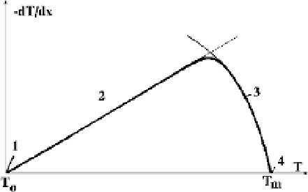
Figure 5.5
The solution of (5.28) for various regions of the thermal wave giving rise to Fig-
ure 5.4.
The solution of this equation for the regions defined in Figure 5.4 is illustrated
in Figure 5.5. Before the thermal wave (region 1) and after it (region 4), we have
Z
0. In region 2 there is no heat release, and one can ignore the last term
in (5.28). This yields
D
u
(
T
T
0
)
Z
D
.
(5.29)
Ignoring the first term in (5.28), we obtain
t
Z
T
m
2
c
p
N
Z
D
f
(
T
)
dT
(5.30)
T
for region 3 in Figure 5.5. Equations (5.29) and (5.30) are not strictly joined at the
interface between regions 2 and 3 because there is no interval where one can ignore
both terms in (5.28). But because of the very strong dependence of
f
(
T
)on
T
,there
is only a narrow temperature region where it is impossible to ignore one of these
terms. This fact allows us to connect solution (5.29) with (5.30) and find the velocity
of the thermal wave.
Introducing the temperature
T
that corresponds to the maximum of
Z
(
T
),
(5.28) gives
f
(
T
)
uc
p
N
.
Z
max
D
Z
(
T
)
D
Equation (5.28) for temperatures near
T
then takes the form
1
.
dZ
dT
D
u
f
(
T
)
f
(
T
)
Solving this equation and taking into account (5.26), we have
u
u
α
Z
D
(
T
T
0
)
exp[
α
(
T
T
)] .
(5.31)