Image Processing Reference
In-Depth Information
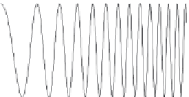
fashion that the spatial frequency is in proportion with the square of the distance from
the center. The waveform from the center to the right edge along the arrow indicated in
Figure 6.5 is shown in Figure 6.6a.
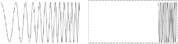
Figure 6.6b shows aperture periodicity, that is, the sampling frequency. To emphasize the
effects, a coarser pitch is chosen, and the aperture ratio
a
/
p
is set at 0.5. As the waveform in
Figure 6.6a is sampled with the pitch of Figure 6.6b, the mathematical forms of Figure 6.6a
and b are multiplied using spreadsheet software. All values except those for the aperture
areas in Figure 6.6b are set to zero. The calculated results are shown in Figure 6.6c and d.
That the amplitude modulation is seen even in a lower-frequency region than the Nyquist
frequency indicates that the amplitude is not reproduced accurately according to the sam-
pling conditions. Figure 6.6c and d in a higher area than the Nyquist frequency show that
the waveforms are false signals completely different from the input signals. Specifically,
Figure 6.6c shows symmetry with the Nyquist frequency at the axis, as the name “folding
noise” suggests.
Reduced by OLPF
(a)
×
(b)
Aperture in pixels
∥
False signal due to aliasing
(c)
Phase 2
Nyquist frequency
(d)
Phase 1
FIGURE 6.6
Model simulation of CZP pattern using spreadsheet software: (a) waveform of CZP pattern input signal;
(b) sampling pitch; (c, d) calculated results.