Environmental Engineering Reference
In-Depth Information
plot
command is applied for a matrix, the values in the
columns are plotted against line numbers. As an exercise check that the command
When the MATLAB
®
produces two function graphs based on four nodes each. In order to obtain a plot of
lines against column numbers one has to use the command for the transpose matrix.
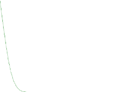
The final command
produces the plot (Fig.
4.2
):
In case of pure diffusion the solution of Ogata & Banks simplifies to the form:
x
2
p
cðx; tÞ¼c
in
erfc
(4.5)
Dt
The dimensionless solution
c/c
in
is identical to the complementary error function
with the dimensionless argument
x ¼ x=
2
D
p
. The evaluation can be performed
easily in the classical manner: if one is interested in the concentration at location
x
and at time
t
, it is convenient to calculate
and to go with the obtained value into
the graphical plot of error function (Fig.
4.1
) to get the corresponding functional
value. The latter has to be multiplied by
c
in
to receive the wanted
c
value.
Exercise 4.1: Heat diffusion
D ¼
x
10
6
m
2
/s,
T
0
¼
5
C,
T
1
¼
15
C,
L ¼
1m;
how long does it take until the temperature on the other side of the wall reaches
1
0.9
0.8
0.7
0.6
0.5
0.4
0.3
0.2
0.1
0
0
5
10
15
20
25
30
35
40
45
50
Fig. 4.2 The solution for the transport equation; analytical solution computed with MATLAB