Environmental Engineering Reference
In-Depth Information
However, it may be sufficient for certain populations for certain time periods. The
most obvious flaw of the model is that it allows the population to increase beyond
any arbitrary margin, provided the time period is long enough. Of course this is
impossible: as soon as a certain high population density will be reached, conditions
will turn to become increasingly unfavourable and the reproduction rate will
become smaller than assumed by the linear approach. Extended model approaches,
which take a
carrying capacity
into account, will be presented in Chap. 19.
Let's examine the situation in which the proportionality constant in the example
given above is lower than 1:
Note that it is allowed to write several commands in a single line, as demonstrated
in the first line. In such a case it is necessary to finish the writing of commands with
;
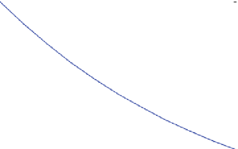
(the last must not have it). Instead of using a negative parameter, we choose to specify
a positive value but write the formula with a minus sign (Fig.
1.7
).
Obviously the population is decreasing. This model is particularly interesting for
biogeochemical species in the environment. In many situations the concentration of
a chemical or biochemical species is declining according to the simple linear
model, as presented. The shown development of concentration is well known as
exponential decay. Exponential decay depends on the linear decay law (
1.12
).
is
called the decay constant or degradation constant, depending on the nature of the
real process.
The proportionality constant can be related to a characteristic half-life
T
1/2
. The
relationship is obtained from the condition:
l
10
9
8
7
6
5
4
3
0
0.1
0.2
0.3
0.4
0.5
0.6
0.7
0.8
0.9
1
Fig. 1.7 MATLAB
figure; second example
®