Environmental Engineering Reference
In-Depth Information
1
analytical
Δ
t=.5
Δ
t=.25
Δ
t=.125
Δ
t = .0625
0.8
0.6
0.4
0.2
0
0
0.2
0.4
0.6
0.8
1
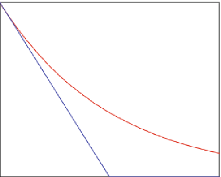
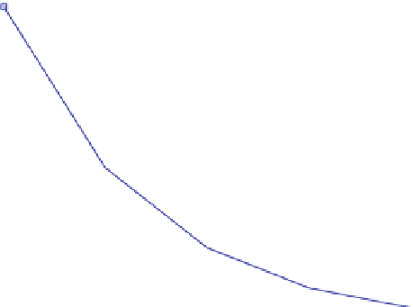
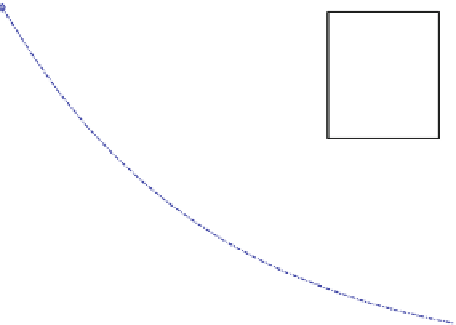
Fig. 21.1 Analytical solution (
red
) and numerical solutions for different timesteps
the wanted accuracy. In the example above, if the modeller is interested in
c
(
t ¼
1),
the following approximations are obtained in 12 refinement steps:
0
0.0625
0.1001
0.1181
0.1268
0.1311
0.1332
0.1343 0.1348 0.1351 0.1352 0.1353 0.1353
If she/he is interested to obtain the first 4 digits of
c
(1) accurate, she/he can stop
the algorithm after the 12th refinement, as the result shows no change in the first
four digits any more.
21.2 Finite Differences
In the previous chapter the numerical method of finite differences has been used for
the approximate solution of the decay equation. The method can in general be used
for the solution of ordinary or partial differential equations. The recipe to replace
differentials by finite differences can be applied for time derivatives and spatial
derivatives in all space directions. In case of spatial differentials we speak of a
grid
spacing
instead of a timestep, and we use the symbols
D
x;
D
y
and/or
D
z
instead
D
t
.
For first order derivatives there are various alternatives; forward, backward and
central FD:
of
@u
@x
u
ð
x
þ
D
x
Þ
u
ð
x
Þ
D
x
forward
@u
@x
u
ð
x
Þ
u
ð
x
D
x
Þ
D
x
(21.9)
backward
@u
u
ð
x
þ
D
x
Þ
u
ð
x
D
x
Þ
2
@x
central