Environmental Engineering Reference
In-Depth Information
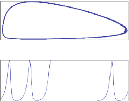
Fig. 19.5 Example output of
a predator-prey model
predator
2
trajectory
1
0
0
0.5
1
1.5
2
prey
2
prey
predator
1
0
0
20
40
60
80
100
time
the lower boundary the predator population remains small, while the prey has
favourable conditions. Then, the number of predators starts to increase, which at
the rightmost positions leads to a decline of the prey. With declining prey the
predator population can increase only for a limited time, until, at the uppermost
position of the closed curve, these decline, too. Finally, near the origin the low
abundance of predators makes the prey population rise again.
The result, obtained by the numerical methods included in MATLAB
,
coincides with findings from analytical methods for the simple and much examined
classical Lotka-Volterra system. In fact, it is easy to see that there are two equilib-
rium solutions:
®
and c
2
¼
0
0
r
2
=a
2
r
1
=a
1
c
1
¼
(19.13)
The Jacobi-matrix can be used to examine the stability of the equilibria. Simple
calculations yield that the eigenvalues of the Jacobi-matrix at c
1
are
r
1
and -
r
2
.As
the second eigenvalue is real and positive, the equilibrium is unstable. At c
2
the
eigenvalues are pure imaginary
r
1
r
p
, which indicates a stable equilibrium
with oscillations around the equilibrium in its vicinity. In the phase space there are
circular motions around the equilibrium. The reader may explore this using the
MATLAB
i
M-file by changing the initial value
c0
.
The solutions in the phase space can also be obtained by integration (Richter
1985, Murray
2002
). In non-dimensional form they are given implicitly by the
equation:
®
r
1
r
2
ln
ðc
1
Þc
1
¼
ð
ln
ðc
2
Þc
2
Þ þ c
0
(19.14)