Environmental Engineering Reference
In-Depth Information
has negative eigenvalues for
r
1
=a
1
>r
2
=a
2
and
positive eigenvalues if the inequality holds in opposite direction. For the Jacobi-
matrix at
The Jacobi-matrix at
ðr
1
=a
1
h
1
;
0
Þ
the conditions are exactly reversed. The analysis shows that
the result, obtained above for the example values from a phase space analysis, is
generally valid.
For the degenerate case with
r
1
=a
1
¼ r
2
=a
2
one eigenvalue becomes zero; as the
other one is negative the equilibrium is still stable. However, it needs to be noted
that all positions on a line are also equilibria in that case. The eigenvalues for those
points are
a
1
h
1
c
1
and
a
2
h
2
c
2
and thus also negative. All these equilibria are
stable.
In order to visualize this in the phase space, various trajectories have been
plotted as described above. Input parameter within the
'compspec.m'
were specified
as follows:
ð
0
;r
2
=a
2
h
2
Þ
T = 1000;
% maximum time
r = [1; 1];
% rates
e = [1; 1];
% equilibria
lambda = 1.;
% lambda parameter
Several starting positions were chosen and the M-file was run several times with
the
hold on
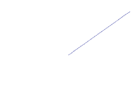
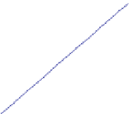
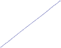
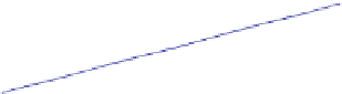
option being active. As shown in Fig.
19.4
all trajectories are straight
lines, which end at the diagonal that connects the upper left and the lower right
corners of the plotted region. Using the mathematical analysis from above it is easy
to verify that this line represents all equilibria (except zero). The illustration allows
the obvious conclusion that the equilibria on the line are stable, which we already
know from the eigenvalues.
1
0.8
0.6
0.4
0.2
tr
a
je
c
to
r
y
0
0
0.2
0.4
0.6
0.8
1
specie 1
Fig. 19.4 Trajectories in the phase space for the degenerate case
0 of the competing species
model; all equilibria on the diagonal line (from
upper left
to
lower right
) are stable
l¼