Environmental Engineering Reference
In-Depth Information
1
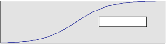
logistic growth
population
0.5
0
0
1
2
3
4
5
6
7
8
9
10
time
Fig. 19.1 Logistic growth; Computed form analytical solution using MATLAB
®
values
c
, for which the left hand side of (
19.1
) vanishes:
f
(
c
)
¼
0. The population
c ¼
0 is an unstable equilibrium, while
c ¼ k
is stable. Small deviations from the
unstable equilibrium, in the example
c
0
¼
0.01, lead to increased deviations at
later times. The user may check easily for the given parameters that an initial value
near to the stable equilibrium of
c ¼
1 produces an almost constant system
development.
The stability of equilibria can be examined by the use of the derivative. For
a negative value of the derivative the system is stable, while it is unstable for
a positive derivative. For the logistic (
19.1
) there is
, which is
positive at the origin but negative for
c ¼ k.
In the following we treat systems
of equations instead of single equations. For systems the eigenvalues of the Jacobi-
matrix take the just described role of the derivative and have to be examined in
order to check the equilibria for stability.
There is almost no branch of environmental modeling in which nonlinear
systems do not appear. In ecological sciences ecosystems are in the focus with
interactions between species populations. The structure of a foodweb model is often
visualized in a compartment graph, in the way hydrological systems were
represented in Figs. 18.1 and 18.2. An example of a foodweb graph is depicted in
Fig.
19.1
. Species or groups of species are represented by compartments. Arrows in
foodweb graphs indicate the direction of the food-chain; in the example lake trouts
consume forage fish, which themselves live on zooplankton.
In the example graph, representing a part of the Lake Michigan aquatic eco-
system, there are four trophic levels. Detritus and phytoplankton are the lowest
level and lake trout alone represents the highest level in this model. Most modeling
efforts of lake eco-systems end up with less than five or six trophic levels. Foodweb
structures can be represented by an adjacency matrix and visualized using the
MATLAB
@f =@c ¼ r
1
ð
2
c=k
Þ
®
gplot
command, as shown in Chap. 18.
In the sequel some simple foodweb models are examined as examples for the
treatment of nonlinear systems by MATLAB
. Analytical solutions can be
obtained for simple networks and interactions only, as for example for the logistic
growth (
19.1
). Therefore, numerical methods will be used for the solution for more
complex set-ups. First we study species of the same trophic level, like in the forage
fish or the zooplankton compartments of Fig.
19.2
.
®