Environmental Engineering Reference
In-Depth Information
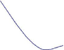
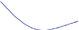
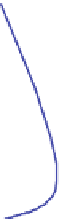
phase diagram
1.5
variable 2
1
0.5
stable
equilibrium
0
variable 1
-0.5
0.5
1
1.5
2
2.5
Fig. 18.8
Phase diagram for a simple compartment model using MATLAB
®
equilibrium similar trajectories result, but the flow direction is opposite. It is left to
the reader to explore these different cases by modifying the
'phasediag.m'
M-file.
Table
18.2
provides a classification of equilibria for a two variable system, based
on the real parts of the eigenvalues (see also: Hale and Ko¸ak (
1991
)
Figure
18.9
provides a view of the stable oscillations that are obtained if both
eigenvalues are purely imaginary, i.e. if both eigenvalues have vanishing real
parts. The trajectories are circles around the origin, describing a cycling of the
corresponding variables: if variable 1 increases, variable 2 decreases and vice versa.
Turning points between these two situations are reached, when one of the variables
has a zero value and changes its sign.
For higher values of
N
the characterization of stable and unstable situations can
easily be extrapolated from the simple
N ¼
2 case. If there is at least one eigenvalue
with a positive real part, the equilibrium is unstable. If real parts of all eigenvalues
are negative, there is convergence towards a stable solution. Degenerate situations,
in which there is at least one purely imaginary eigenvalue, can be interpreted
analogously to the five lower rows in Table
18.2
.
For 2D phase space calculation and visualization,
M-file
'pplane.m'
by Polking is available on the web (
http://math.rice.edu/~dfield/
). It
sets up a graphical user interface (GUI) and has several other convenient features.
The manual for the program is available as a topic (Polking
2004
). We demonstrate
an application example in Chap. 19.
the MATLAB
®