Environmental Engineering Reference
In-Depth Information
1.8
1
2
1.6
1.4
1.2
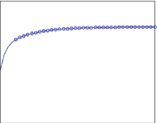
Eigenvalues:
-3.4142 -0.58579
1
0.8
Steady state:
1.5 0.5
0.6
0.4
0
2
4
6
8
10
time
Fig. 18.7
Transient and steady state solution of a two-compartment model using MATLAB
®
(numbers) are converted to strings (command
num2str
), and the result is added
to the figure.
It was already mentioned above that the formula
C
1
f
i
represents the steady
equilibrium. That term is evaluated within the last
text
statement. The transient
development, depicted in the figure, shows that the steady state, obtained by the
evaluation of the formula, is approached. We are in the lucky position that the
steady state can be obtained in two ways: by evaluating an analytical formula and
by regarding the temporal development at long times. In many other models only
the second alternative is available.
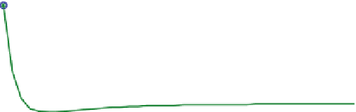
The development of the transient simulation against the steady state (here
(1.5, 0.5)
T
) does not become as obvious as in Fig.
18.7
, if the time interval is
not sufficiently long. Note that there are systems which do not approach the
equilibrium, independent of the length of the time interval. In that case we speak
of an
unstable equilibrium
. It can also be checked by the sign of the biggest
eigenvalue (see below), whether the system converges towards a steady state, i.e.
if the equilibrium is stable or unstable. For the next sub-chapter keep in mind that in
the example the maximum eigenvalue is
c
¼
0.59, and thus negative.
The complete code is included in the accompanying software under the name
“comparts.m”