Environmental Engineering Reference
In-Depth Information
1
35
0.9
30
0.8
25
0.7
20
0.6
0.5
15
0.4
10
0.3
5
0.2
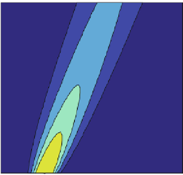
Concentration
0.1
0
-0.05
0
0.05
0.1
0.15
0.2
space
Fig. 16.3 Transport solution for an instantaneous source, represented in a time-space diagram
(see also: Hunt
1983
; Kinzelbach
1987
). Linear equilibrium sorption can be
included following the derivations in Chap. 6. For a constant retardation coefficient
R,
the solution is given by:
!
2
4
tD=R
lt
M
4
ð
x
vt
=
R
Þ
p
cðx; tÞ¼
p
D=R
exp
(16.8)
pt
In analogy to the 1D situation analytical solutions can be derived for the higher
dimensional cases. The generalization of the 1D normal distribution (
16.1
) for
2D is:
"
#
!
2
2
y
m
y
s
y
1
1
2
x
m
x
s
x
f ðx; yÞ¼
exp
þ
(16.9)
2
ps
x
s
y
with standard deviations
m
y
for
x
- and
y
-directions. Formula (
16.9
) gives the solution of the differential equation
s
x
and
s
y
and mean values
m
x
and
@
c
@t
¼
@
@x
D
x
@c
@x
þ
@
@y
D
y
@
c
(16.10)
@y
with a
m
y
) and zero
boundary condition at infinity. Standard deviations and diffusivities are related
by the equations
-peak initial condition (formula (
16.3
)) at position (
m
x
,
d
p
2
D
x
t
2
D
y
p
.
s
x
¼
and
s
y
¼