Environmental Engineering Reference
In-Depth Information
The conjugate complex is denoted by an over bar and defined as follows:
z ¼ x iy
(15.12)
In MATLAB the conjugate complex of a complex number
z
is calculated by
using the
conj
function:
Often it is easier to implement the imaginary potential instead of the separate
computation of the real potential and the streamfunction (see examples in Table
15.2
).
When the complex potential is computed, (real) potential and streamfunction can be
obtained as real and imaginary part of the imaginary potential:
' ¼
Re
ðÞC ¼
Im
ðÞ
(15.13)
There are more analytical elements than those for baseflow and wells. Formulae
for line sinks or line sources, for di-poles, for vortices and so forth can be found in
the textbooks.
Table 15.2 Complex potentials for various flow patterns; basic flow patterns with parameters as
1
2
z
1
þ
z
ð
z
2
Þ
in Table
15.1
; with Z
¼
1
2
ð
z
2
z
1
Þ
Element
(Imaginary) Potential
F
Q
0
z
Baseflow
Well
Q
2
log
ð
z
z
well
Þ
p
A
pi
Vortex
log
ð
z
z
0
Þ
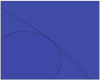
Di-pole
s
2
p
exp
ðibÞ
z
z
0
n
h
i
o
Line-sink
6
s
L
4
Þ
2 log
1
2
ð
Z
þ
1
Þ
log Z
þ
1
ð
Þ
Z
1
ð
Þ
log Z
1
ð
ð
z
2
z
1
Þ
2
p
Fig. 15.8 Dipole pattern
(streamlines white, potential
contours black)
6
Between positions z
1
and z
2
with strength
s.