Environmental Engineering Reference
In-Depth Information
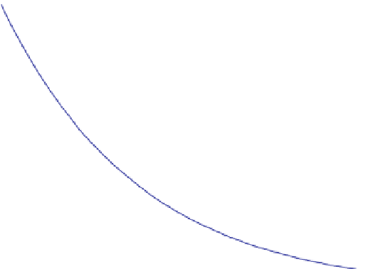
0.8
given
modelled
0.7
0.6
λ
: 0.33287
0.5
norm of residuals: 0.064604
0.4
0.3
0.2
0.1
0
0
1
2
3
4
5
6
7
8
Fig. 10.5 Exponential fit for parameter
l
using the demonstration data set
In the following M-file the zero of that function is determined. The sum of
(
10.13
) is evaluated in the last line. In all other parts the M-file resembles the
'par_est.m'
example given above.
function par_esta
% parameter estimation with derivatives
% for exponential fit for c0
global tfit cfit lambda
% specify fitting data
tfit = [0.25 1 2 4 8];
cfit = [0.7716 0.5791 0.4002 0.1860 0.1019];
lambda = .3329; c00 = 1.;
c0 = fzero(@myfun,c00);
normc = norm(cfit - c0*exp(-lambda*tfit));
display (['Best fit for c0= ' num2str(c0)]);
display (['Norm of residuals= ' num2str(normc)]);
tmax = tfit(size(tfit,2));
t = [0:0.01*tmax:tmax];
figure; plot (tfit,cfit,'or',t,c0*exp(-lambda*t),'-');
legend ('given','modelled');
text(0.5*tmax,c0*0.7,['c_0: ' num2str(c0)]);
text(0.5*tmax,c0*0.8,['norm of residuals: ' num2str(normc)]);
function f = myfun(c0);
global tfit cfit lambda
c = c0*exp(-lambda*tfit);
%solve linear decay equation for c with c(0)=c0
cc0 = exp(-lambda*tfit); % equation for dc/dc0
f = (c-cfit)*cc0'; % specify function f to vanish