Environmental Engineering Reference
In-Depth Information
Table 8.4 Parameter for calcite dissolution simulation (CAL - see: Saaltink et al
.
2001
)
Variable
Value
Unit
Initial concentration
TotH
7.978
log mol/l
Initial concentration
TotC
3.018
log mol/l
Initial concentration
TotCa
3.019
log mol/l
Inflow concentration
TotH
5.496
log mol/l
Inflow concentration
TotC
5.421
log mol/l
Inflow concentration
TotCa
4.398
log mol/l
9.939 10
4(1)7
Kinetic transfer coefficient(s)
mol/(l a)
10
9
8
MatLab,CAL-1
MatLab,CAL-2
MatLab,CAL-3
MatLab,CAL-4
MatLab,Cal-E
7
6
0
20
40
60
80
100
distance[m]
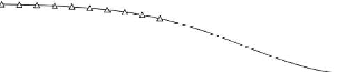
Fig. 8.3 Calcite dissolution example; results for different calcite dissolution kinetics
Figure
8.3
illustrates the results for pH in dependence of the kinetic transfer
coefficient. For the cases CAL-1-CAL-4, the kinetics rate is increased by a factor of
10, taking the values given in Table
8.4
. In the CAL-1 case, the process of calcite
dissolution is too slow to have any effect on pH. There is a front of low pH
penetrating the system.
For enhanced kinetics the already mentioned rise of pH becomes more and more
pronounced. Due to increased calcite disolution, H
+
ions are increasingly consumed
by the dissolved carbon species. As a result, the pH is increased where the inflowing
water dominates. The equilibrium situation is approached gradually with a front of
high pH entering the fracture.
The MATLAB
simulation is again based on a combination of the
pdepe
solver
and speciation calculations based on the Newton method. Holzbecher (
2006
)
extended the presented approach for the simulation of the horizontal and vertical
concentration distribution within a fracture. The 2D flow field is computed follow-
ing the Hagen-Poiseuille analytical solution (see Chap. 11). The 2D advection-
®