Environmental Engineering Reference
In-Depth Information
The computations for variables
h
and
u
have to be extended:
Then the explicit formula is written as follows:
That's all. Let's examine some solutions calculated with the extended code.
The complete code is included in the accompanying software under the name
'analtrans.m'.
Exercise 6.1:
Compare results with
R ¼
1 and
R ¼
3, with parameters:
T ¼
1,
v ¼
0!
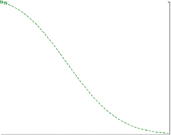
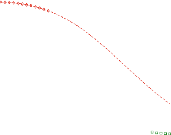
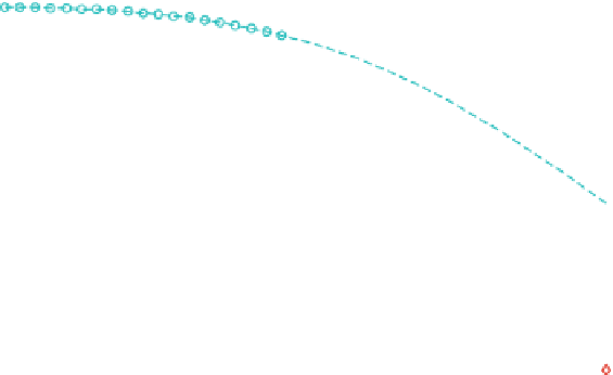
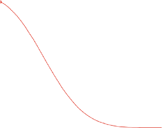
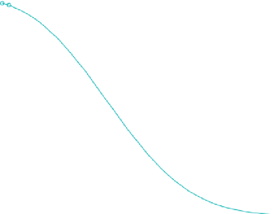
Figure
6.3
depicts the results for exercise 6.1. The effect of retardation is nothing
but a factor in the time-scale. The concentration distribution at time
tR
for the
retarded species is identical to the curve at time
t
for the tracer - at least that is the
1,
D ¼
0.1,
L ¼
1,
l ¼
1
0.9
0.8
0.7
0.6
0.5
0.4
0.3
0.2
0.1
0
0
0.1
0.2
0.3
0.4
0.5
0.6
0.7
0.8
0.9
1
space
Fig. 6.3
Result of exercise 6.1; both situations are represented by three concentration
distributions. Squares mark
t ¼
1/3, diamonds
t ¼
2/3 and circles
t ¼
1. The graph for
R ¼
1
and
t ¼
1/3 falls together with the graph for
R ¼
3 and
t ¼
1