Environmental Engineering Reference
In-Depth Information
1
solid phase concentration
0.9
0.8
0.7
0.6
0.5
0.4
linear
Freundlich
Langmuir
0.3
0.2
0.1
fluid phase concentration
0
0
0.1
0.2
0.3
0.4
0.5
0.6
0.7
0.8
0.9
1
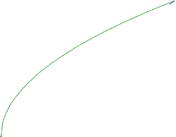
Fig. 6.2
Illustration of sorption isotherms: linear, Freundlich and Langmuir
4
Table 6.2
Overview on further sorption isotherms
Sorption isotherm
Formula
Number of parameters
Linear
c
s
¼ K
d
c
1
c
s
¼ a
F
1
c
a
F
2
Freundlich
2
a
L
1
c
a
L
2
þ c
Langmuir
c
s
¼
2
Tempkin
c
s
¼ a
T
1
þ a
T
2
log
ðcÞ
2
Frumkin
2
K
d
exp 2
a
F
cð Þc
1
þ K
d
exp 2
a
F
c
s
c
s
¼
ð
Þc
a
1
c
a
3
a
2
þ c
a
3
Langmuir-Freundlich
3
c
s
¼
a
1
c
a
2
þ c
a
3
c
s
¼
Redlich-Petersen
3
a
1
c
a
2
þ c
a
3
Toth
c
s
¼
3
1
=a
3
ð
Þ
Dubinin-Raduskevich
1
log
2
3
log
cðÞ¼a
2
ðÞþ
a
log
ðÞ
a
3
A very popular description for the equilibrium between the cations is the
Gapon
isotherm:
c
s
1
c
2
1
=n
2
c
s
2
c
1
1
=n
1
¼ K
(6.8)
4
produced using MATLAB
by:
c
¼
[0:0.01:1]; cs1
¼
c; cs2
¼
c.^0.5; cs3
¼
3*c./
(1 + 2*c); plot (c,cs1,c,cs2,c,cs3);
and some additional design changes from the Figure
editor.
®