Transport with Decay and Degradation - Environmental Modeling - page 96

c ¼ c 0 exp ð l tÞ (5.4)

which holds for the initial condition c ( t ¼

¼ c 0 . The exponential function
obviously is the solution for a component with first order decay - that explains
the notation exponential decay .
The half-life t ½ is the time period in which the component concentration declines
to half of the initial value. Thus according to ( 5.4 ) the t ½ is characterized by the
condition

0)

1 = 2 ¼ exp ð l t 1 = 2 Þ (5.5)

which is equivalent to the condition t 1 = 2 ¼ . This is the reciprocate relation

between decay constant and half-life. With t ½ exponential decay can be noted in
dimensionless form as:

ln ð 2 Þ= l

c
c 0 ¼

t
t 1 = 2 Þ

exp ð ln ð 2 Þ (5.6)

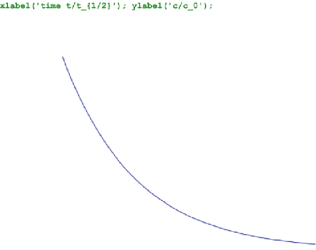
for the dimensionless variables c / c 0 and t / t ½ . For the time period of five half-lifes
the function is depicted by the following MATLAB ® commands in Fig. 5.2 .

1

0.9

0.8

0.7

0.6

0.5

0.4

0.3

0.2

0.1

0

0 1 2 3 4 5

time t/t 1/2

Fig. 5.2 Exponential decay as represented by dimensionless variables