REACTORS: IDEALIZED CHEMICAL REACTORS - Biomass as a Sustainable Energy Source for the Future - page 169

dV (m 3 )
d X A

c A0 mol.m -3

c A f mol.m -3

φ n , A

φ n , A 0 mol.s -1

φ n , A +d φ n , A

φ n , Af mol.s -1

X Af (-)

X A 0 =0

X A X A +d X A

φ Vf m 3 .s -1

φ V0 m 3 .s -1

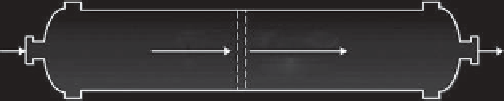
FIGURE 6.3 Plug flow reactor.

the plug flow model mathematically, it is common to divide the total volume
of the reactor in an infinite number of slices, infinitely thin and with constant
concentration (Figure 6.3).
The steady-state molar balance around each slice of the reactor is

Rate of accumulation = rate of supply − rate of release + rate of production )

+dV

0= φ n , A − φ n , A +d φ n , A R ð Þ − ð Eq : 6 : 23 Þ

After simplification, the balance reads

d φ n , A = R ð Þ − dV ð Eq : 6 : 24 Þ

Using the definition of conversion,

φ n , A = φ n , A 0 1 X ð Þ − ð Eq : 6 : 25 Þ

Differentiation of Equation (6.25), substitution in Equation (6.24), and rearrangement
lead to

= ð

X Af

V
φ n , A 0

d X A
−

ð Eq : 6 : 26 Þ

R ð Þ

0

Comparing Equations (6.19) and (6.26), we observe that in the CSTR there is no need
of integrals (resulting in a relatively simple algebraic equation) because the term
( R A ) is constant throughout the whole reaction volume, whereas in the PFR, the

conversion changes with the axial position, so (

−

R A ) also changes.
If the kinetics of the reaction is known Equation (6.26), allows calculation of the
volume of the reactor necessary for a conversion X A of a flow

−

φ n , A 0 of reactant A. The

time τ needed to process one reactor volume of feed can be calculated as

=c A0 ð

X Af

= V
φ V 0

= Vc A0
φ n , A 0

d X A
−

τ for any ε A ð Eq : 6 : 27 Þ

R ð Þ

0