Application of Electrokinetics for Enhanced Oil Recovery - Electrokinetics for Petroleum and Environmental Engineers - page 116

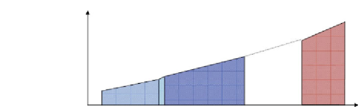
Melting

Joule-Heating

Electro-Kinetic
Mass Transport

Electrochemical

Figure 3.7 Schematic representation of the energy requirements of various electrokinetic
mechanisms and electrical melting (after Wittle et al., 2008c)

All of the above five mechanisms are coupled reactions. Nourbehecht
and Madden (1963), as well as Mitchell (1993) provide simple linear alge-
bra and tensor representations.
In matrix notation, Onsager's relationships can be represented as:

J
J
J
J
J
J

LLLLLL
LLL

∇
∇
∇
∇

f
f
f
f 4

⎡ ⎤ ⎡ ⎤ ⎡ ⎤ 1 11 12 13 14 15 16 1

⎢
⎢
⎢
⎢
⎢
⎢
⎢
⎢

⎥
⎥
⎥
⎥
⎥
⎥
⎥
⎥

⎢
⎢
⎢
⎢
⎢
⎢
⎢
⎢

⎥
⎥
⎥
⎥
⎥
⎥
⎥
⎥

⎢
⎢
⎢
⎢
⎢
⎢
⎢
⎢

⎥
⎥
⎥
⎥
⎥
⎥
⎥
⎥

LLL
LLLLLL
LLLLLL
LLL 54

2 21 22 23 24 25 26 2

3 31 32 33 34 35 36 3

(3.2a)

=

4 41 42 43 44 45 46

LL
LLLLLL

∇
∇

f
f

5 51 52 53 55 56 5

⎣ ⎦ ⎣ ⎦ ⎣ ⎦

6 61 62 63 64 65 66 6

.

or, using the simpler tensor notation, they are:

6

∑ 1

. (3.2b)

J = L ∇ f

i ij j

j

where: J i are generalized flow, or flux vectors.

Ø j are generalized potential gradient, or force, vectors.
L ij are generalized conductivity, or coupling coefficient (second
rank) tensors.
The direct flow, or main diagonal terms, L ii , of Equation 2a relate non-
coupled fluxes to their potential gradients, whereas the off diagonal terms,
L ij , relate coupled fluxes.
Reviewing Equations 3.2a and 3.b2b, one can observe that:

∇

• If J 1 is electrical current density and Ø 1 is electrical poten-
tial, then L 11 is the electrical conductivity tensor, σ , whereas