Mud Siren Torque and Erosion Analysis - Measurement While Drilling Signal Analysis, Optimization and Design - page 188

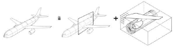
Figure 7.7. Three-dimensional mean surface approach.
7.3 Mud Siren Formulation
Aerospace engineering experience shows that small geometric details -
say, contours selected for airfoils and ailerons - greatly affect aerodynamic
performance, e.g., changes to quantities like moment, pressure distributions, lift,
flow separation point, pitch stability, and so on. End results are not apparent to
the naked eye and must be modeled rigorously. For instance, the radically
altered behavior going from Figure 7.1 to Figure 7.2 arose principally from the
effect of small streamwise rotor tapers, whose end effects could not have been
anticipated a priori. One can only surmise the effects of different combinations
of tapers in stators, rotors, and upstream and downstream annular passages.
Practical computational concerns require geometric simplification, but
these cannot be made at the expense of incorrect physical modeling. In this
section, we adopt the philosophy suggested in Section 2, namely, that geometric
boundary conditions can be successfully modeled along mean lines and surfaces
while retaining the three-dimensional partial differential equation in its entirety,
as suggested in Figure 7.7. With this perspective and philosophical orientation,
we correspondingly assume a cylindrical coordinate system for analysis, that is,
the ones implied by Figures 7.8 and 7.9.
From aerospace analogies, we expect that the torque acting on the siren
lobe (again, perpendicular to the direction of flow) can be accurately predicted
since it is inviscidly dominated and is largely independent of shearing and
rheological effects. This is particularly so because strong areal convergence at
the lobes precludes local separation. On the other hand, viscous pressure drops
in the streamwise direction and downstream separated flows cannot be modeled
using inviscid theory. With these limitations in mind, we proceed with a
comprehensive three-dimensional formulation.
7.3.1 Differential equation.
In cylindrical radial coordinates, Laplace's equation 2 I= 0 takes the
form given by
I xx + I rr + 1/r I r + 1/r 2 I TT = 0 (7.3.1)
where x is the axial streamwise variable, r is the radial coordinate, and T is the
azimuthal angle. It is possible to solve this three-dimensional partial differential