Environmental Engineering Reference
In-Depth Information
A
B
Height (cm)
Height (cm)
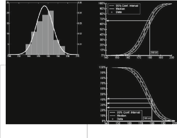
Panel A.
Example of a histogram (bar graph) and a probability
density function or PDF (the curve), showing the variation
in height of people attending a workshop
Panel B (same data).
The cumulative distribution function (CDF), showing the variation
in height of people attending a workshop. The central curve is a
parametric CDF (fitted Normal distribution); the points represent
the original data (empirical CDF); and the outer curves show the
CDF. The arrow shows how to estimate the proportion of the
population with heights below any given value.
Panel C (same data)
Example of an exceedance function (EXF), showing the variation
in height of people attending a workshop. The central curve is a
parametric EXF (fitted Normal distribution); points and outer
curves like in panel B. The arrow shows how to estimate the
proportion of the population with heights above any given value,
together with a 95% confidence interval
C
parametric CDF (fitted Normal distribution); the points represen
95% confidence interval for the sampling uncertainty of the fitted
Height (cm)
Fig. 14.3
By creating a distribution (either a bell-shaped probability density model,
panel a
)or
either of the two possible sigmoid cumulative models (
panel b
and
c
), one can summarize the key
characteristics of a data set, and derive consequences of certain conditions imposed on the entities
composing this data set. From EUFRAM (
2006
)
The fitted models allow for summary of the raw data in a few parameters, like
the mean and the variance for the Normal distribution.
If this particular “sample of visitors” were gathered in a room with a door height
of 180 cm, the most basic interpretation (based on raw data on height of people
and the door) is that exactly those people with lower height could safely leave the
room without hitting the top of the door frame. From the summary models, one
can calculate that 68% of the people would be safe from hitting the top of the door
frame when leaving the room (panel B), or that 32% would be unsafe (panel C).
The summary models can be used in a subsequent workshop to predict the people
“at risk”. In such a case, the representativity of the measured sample of people is
relevant, as well as the sample size. When the sample size increases, the uncertainty
of the prediction is commonly reduced. This reduction of statistical uncertainty is
captured in the confidence intervals shown in panels B and C. What remains is the
uncertainty that the sampled people are not representative for assessing the risks for
participants of other workshops in the same room.
The sigmoidal cumulative distribution, Panel B, was originally adopted to rep-
resent the SSD concept in ecotoxicology mostly in Europe (other authors prefer a
linear probit model). Using a curve like Panel B, a community could be assumed
protected against adverse effects of contaminant exposure by deriving an estimated
Search WWH ::

Custom Search