Fundamentals of Digital Image Processing - Control of Color Imaging Systems: Analysis and Design - page 33

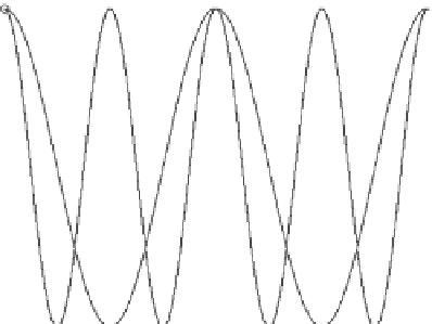
f a ( x ): Original analog signal

Reconstructed signal

= Signal samples

1
f s

1

=

Δ x =

300

x

Δ x 2Δ x 3Δ x 4Δ x 5Δ x 6Δ x

FIGURE 2.11 One-dimensional example of aliasing.

The signal has frequency components of 200 and 300 cycles per unit length in
the

x- and y-directions, respectively. Thus the Nyquist rate for the signal is

f Nyquist ¼ (400, 600) cycles per unit length. To avoid aliasing,

the sampling rate must exceed the Nyquist rate. Now suppose we sample the
signal at a rate below the Nyquist frequency, say 300 and 400 samples per unit
length in the x- and y-directions, respectively. Then the sampled signal is

2 (200, 300) ¼

400 p

300 nþ

600 p

400 m

4 3 nþ 3 2 m

f (n, m) ¼ 2 cos

¼ 2 cos

4 3 n 3 2 m 2 3 n 2 m

¼ 2 cos 2 pnþ 2 pm ¼ 2 cos

2 3 nþ 2 m

¼ 2 cos

Now, if we send the sampled signal through an ideal digital to analog converter
(D

= A), the resulting continuous signal would be

2 3

300x þ 2 g(x, y) ¼ 2 cos 400y ¼ 2 cos (200 pxþ 200 py)

This means that the reconstructed signal appears as a low-frequency signal.

Example 2.3

To show aliasing in an image, we first downsample the monochromic LENA image

shown in Figure 2.12a by a factor of 4 and then upsample it to the original size
without using any anti-aliasing filter. The resulting image is aliased as shown in

Figure 2.12b.