Internal Process Controls - Control of Color Imaging Systems: Analysis and Design - page 482

0

-50

-100

-150

-200

-250

-300

-350

-400

-450

2 4 6 8 10 12 14 16

X (ergs/cm 2 )

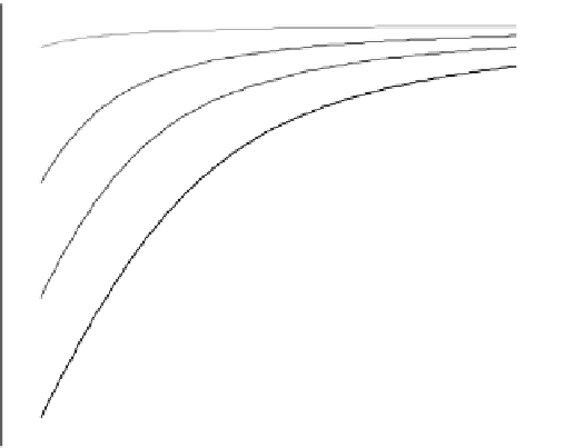
FIGURE 9.7 X(U l ) - V l curves for V g (U g ) ¼ [ 300 V (upper curve), 500 V, 600 V, 700 V

(lower curve)].

S OLUTION
The controllability matrix (Equation 4.121) is given by

0 : 9798 0 0 : 9798 0

Q ¼ [BAB] ¼

0 : 3315 11 : 1026 0 : 3315 11 : 1026

Since the rank of the controllability matrix is two, the electrostatic system is fully
controllable at the nominal operating point. Since A is identity matrix, the same
conclusion can be reached by finding the rank of the Jacobian matrix (B).

9.4.1 E LECTROSTATIC C ONTROLLER D ESIGN
From the theory of linear systems, it is known that two of the most important properties
to examine before designing a controller are controllability and observability (see
Chapters 4 and 5). We now check these conditions for the LTI system of Equation
9.21. While observability is, by de nition, guaranteed, since the output is equal to the

state vectors (C find a condition for controllability. Since A ¼ I, this

condition is trivial and simply requires that matrix B is full rank. This is an important
condition for control to be successful and is usually satis

¼ I), we need to

ed everywhere except at the

boundary limits of the actuators. If this is satis ed, then state-feedback control

(equivalent to output-feedback control in this case) is feasible and arbitrary pole
placement of the closed-loop system can be carried out via many techniques through
the appropriate selection of the feedback gain matrix K (see Figure 9.1).