Interpolation of Multidimensional Functions - Control of Color Imaging Systems: Analysis and Design - page 283

1.2

0.8

0.4

0.2

0

0 0.2 0.4 0.8 1.2

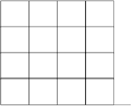
FIGURE 6.20 Grid locations for 2-D example.

Example 6.10

Consider the following 3-D nonlinear function:

¼ x þ x 2 5y 1:6 þ xy 4

f f(x, y, z) þ xy þ 1 : þ 0 : 10 x, y 1

The function f(x, y, z) is uniformly sampled with Dx ¼Dy¼Dz¼ 0.25 over a cube

of size [0 1] 125 samples. The

3-D DO algorithm is used to downsample the LUT to a smaller LUT of size
3

[0 1] [0 1], generating a LUT of size 5 5 5 ¼

27 samples. The resulting MMSE is 1.1107 and the optimal grid points
are shown in Table 6.14.

3 3 ¼

Example 6.11

The overall system for constructing a three-to-three inverse LUT with reduced
patch measurements is shown in Figure 6.21 The system performance is measured
in terms of the error between the mapped input and output L*a*b* values:

*

E ¼ L*a*b out Lab in (mapped) (6 : 75)

The forward printer model P is constructed by printing 13 3 uniformly sampled,
CMY color patches and measuring their L*a*b* values using a spectrophotometer.
This LUT is then downsampled to 3, 4, . . . , 13 cubes and then upsampled to the
original size (13 cubes). Applying ICI to the newly formed upsampled LUT forms
the three-to-three inverse LUT. The 240 test patches that are used to evaluate
the overall system performance consist of 216 patches inside the printer gamut
and 24 patches inside and on the neutral axis (a* 0) of the printer gamut.

The simulation results for a commercial Xerox printer are shown in Table 6.15. As
can be seen, a mean

¼b* ¼

DE 2000 ¼ 0.76 is achievable with the reduced measurements

of size 125 optimal colors.