Interpolation of Multidimensional Functions - Control of Color Imaging Systems: Analysis and Design - page 281

interpolated and original grid point values is minimized. Let the optimal indices be li, i ,
m j , and n k with an MSE of E ijk . In the second stage, we need to find two grid points

within the same cube in order to minimize the MSE as in stage one. If the solution for
the first point has indices l1i, 1i , m 1j , and n 1k , then the total MSE is given by

¼ E ( i, j, k ) þ E l 1i m 1j n 1k

E 2 l 1i , m 1j , n 1k ( 6 : 74 )

where E(i, j, k) is the interpolation error between the original and the interpolated
functions with the cube extending from grid point {ijk} to grid points l1i, 1i , m 1j , n 1k .
Now, we minimize E 2 with respect

to the indices l1i, 1i , m 1j , and n 1k . Note that

the solution to the finding the optimal solution in the second

stage, similar to 1-D and 2-D algorithms. We continue this process until we

first stage is used for

nd the

solution to the N-stage problem. Note that while finding the solution to the N-stage

grid allocation problem, we obtain the solution to all stages up to and including N.

Example 6.8

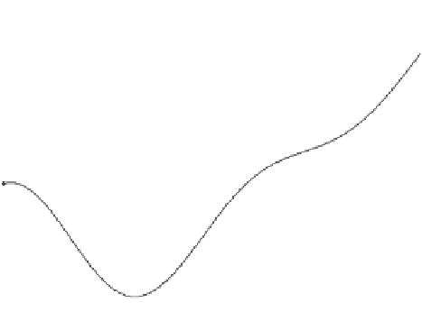
Consider the 1-D nonlinear function shown in Figure 6.18. We apply uniform
sampling, SLI, and DO algorithms to select 5, 6, . . . , 20 grid points. We then use
linear interpolation and interpolate to the original size of the function and com-
pute the MSE between the original function and the upsampled version of the
downsampled function. Figure 6.19 shows the MSE as a function of grid size for
three different algorithms (uniformly sampling with reduced samples and SLI). As
can be seen, the DO algorithm outperforms the other two algorithms.

No n linea r functi o n

1

0.8

0.6

0.4

0.2

0

0 0.1 0.2 0.3 0.4 0.5 0.6 0.7 0.8 0.9 1

x

FIGURE 6.18 Nonlinear 1-D function with eight grid points optimally selected by the DO

algorithm.