Interpolation of Multidimensional Functions - Control of Color Imaging Systems: Analysis and Design - page 250

Example 6.1

Consider the 1-D LUT given in Table 6.2. Use linear interpolation to interpolate
the value of the function at x ¼ 5.4.

S OLUTION
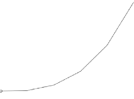
Figure 6.2 shows the plot of function y¼ f(x). As seen from this gure, we have

y i þ 1 y i
x iþ1 x i

3 : 3 1 : 62

y ¼ ð x x i Þ y i ¼ (5 : 4 6) þ 3 : 3 ¼ 2 : 796

6 4

In the 2-D case, the underlying function is a function of two variables, z ¼ f(x, y),
and the nodes in the LUT are uniformly spaced on grids, as shown in Figure 6.3.
Assume that we would like to interpolate the value of the function z at point a with
coordinates (x, y). Let point a be within the grids b - e as shown in Figure 6.4. Then
the bilinear interpolated value of the function at point a is given by

z ¼ f ( x, y ) ¼ p 00 þ tp 01 p 00 ð Þ þ up 10 p 00 ð Þ þ tu p 11 p 01 p 10 p 00 ð Þ ( 6 : 3 )

where
u and t are the relative distances from the surrounding nodes
p 00 , p 01 , p 11 , and p 10 are the values of the function f(x, y) at points b, c, d, and e,
respectively, as shown in Figure 6.4.

TABLE 6.2
Example of a Uniform LUT

x 0 2 4 6 8 10

y 0.9 0.98 1.62 3.3 6.5 11.8

12

10

8

6

4

2

0

0 1 2 3 4 5 6 7 8 9 10

x

FIGURE 6.2 Plot of function f(x).