Information Technology Reference
In-Depth Information
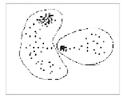
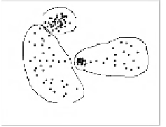
(a)
(b)
(c)
(d)
Fig. 6.20 An example of clustering solutions for a particular dataset. Children
usually propose solution b) and adults solutions b) and c). Solution d) was never
proposed in the study reported in [201].
6.4.4.1
The LEGClust Dissimilarity Matrix
Let us consider the set of objects (points) depicted in Fig. 6.21. These points
are in a square grid in two-dimensional
3
space
x
1
-
x
2
, except for point
Q
.Let
us denote:
•
K
=
{k
i
}
,
i
=1
,
2
, .., M
, the set of the
M
nearest neighbors of
Q
;
•
d
ij
, the difference vector between points
k
i
and
k
j
,
d
ij
=
k
j
−
k
i
for all
i, j
=1
,
2
, .., M
,
i
=
j
. These are the
connecting vectors
between those
points and there are
M
(
M
1) such vectors;
•
q
i
, the difference vector between point
Q
and each of the
M
-nearest neigh-
bors
k
i
.
Despite the fact that the shortest connection between
Q
and one of its neigh-
bors is
q
1
we clearly see that candidates for "ideal connection" are those
connecting
Q
with
P
or with
R
because they reflect the local structure of the
data.
Let us represent all
d
ij
connecting vectors translatedtoacommonorigin
as shown in Fig. 6.22. We call this an
M-neighborhood vector field
.Sincewe
have a square grid, there are a lot of equal overlapped vectors.
−
3
For simplicity we use a two-dimensional dataset, but the analysis is valid for
higher dimensions.