Information Technology Reference
In-Depth Information
4. Update at each iteration,
m
, the parameters
w
(
m
)
k
using a
η
amount (learn-
ing rate) of the gradient:
w
(
m
−
1)
k
∂ R
EXP
∂w
k
w
(
m
)
k
=
w
(
m−
1)
k
−
η
.
(5.42)
5. Go to step 2, if some stopping criterion is not met.
We thus obtain, in the same line as for
R
ZED
,an
O
(
n
) complexity algorithm.
In the following example we apply Algorithm 5.2 to the training of a per-
ceptron solving a two-class problem. In Chapter 6 we describe various types
of (more complex) classifiers using the
R
ZED
and
R
EXP
risks and present a
more complete set of experiments and comparisons with other approaches.
0.0222
x
2
^
E
(e)
2
0.0221
1
0
0.0221
−1
0.0221
−2
x
1
e
−3
0.022
−2
0
2
4
−2
−1
0
1
2
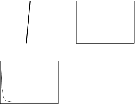
Error Rate (Test) = 0.060
−3350
0.8
Error Rate
^
EXP
−3400
0.6
−3450
0.4
−3500
0.2
−3550
0
0
20
40
60
80
0
20
40
60
80
epochs
epochs
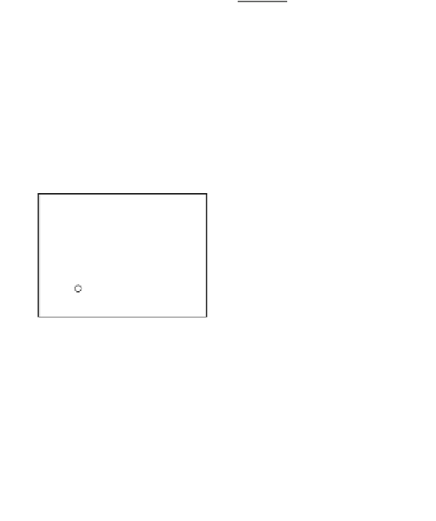
Fig. 5.9
The final converged solution of Example 5.6 with
τ
=
−
18
.
Example 5.6.
Consider the same two-class problem of Example 5.4 (same
data), now solved by a perceptron minimizing the
R
EXP
risk. We consider
two values for
τ
:
τ
=
−
18 and
τ
=2. Recall from formula (5.34) that min-
R
EXP
with
τ
=
−
imizing
18 is equivalent to maximize a scaled version of
R
ZED
with
h
=3. Figs. 5.9 and 5.10 show the final converged solution after
80 epochs. We point out the fast convergence of
R
EXP
(in about 30 epochs)
R
ZED
in Fig. 5.4 with its
R
EXP
version in Fig. 5.9.
mainly when we compare
R
EXP
reaches a good solution in terms of generalization.
Moreover,