Information Technology Reference
In-Depth Information
10
τ
=0.2
τ
=0.5
τ
=1
ψ
Exp
0
e
−10
−1
0
1
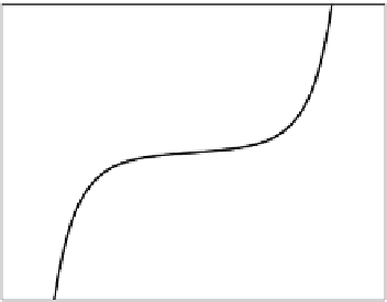
Fig. 5.8
Plot of
ψ
Exp
for different
τ>
0
.
R
ZED
can be seen as a special case of
R
EXP
if we consider
τ<
0.
that is,
R
EXP
gradient behaves like the MSE counterpart. Since
Thus, for
τ
→−∞
,
e
i
=
t
i
−
y
i
, the partial derivative with respect to some parameter
w
is given
by
e
i
exp
e
i
τ
∂y
i
∂w
n
∂ R
EXP
∂w
=
−
2
.
(5.35)
i
=1
Defining as before for formulas (5.23) the weight function
ψ
EXP
(
e
)=
e
exp
e
2
τ
,
(5.36)
we can graphically analyze the behavior of the
R
EXP
gradient. As Fig. 5.8
shows, when
τ>
0,
ψ
EXP
behaves in a similar way to
ψ
CE
.Fromsmallto
moderate values of
τ
, the function has a marked hyperbolic shape: smaller
errors get smaller weights with an “accelerated” trend when the errors get
larger. Note again that lim
τ→
+
∞
ψ
Exp
=
ψ
MSE
. In conclusion, with
R
EXP
we obtain a parameterized risk functional with the flexibility to emulate a
whole range of behaviors, including the ones of
R
ZED
,
R
MSE
and
R
CE
.
The multi-class version of
R
ZED
is given by
1
τ
τ
exp
e
i
e
i
τ
=
n
n
c
R
EXP
=
e
ik
τ
exp
,
(5.37)
i
=1
i
=1
k
=1
where
e
ik
is the error at the
k
-th output produced by the
i
-th input pattern.
Formula (5.37) resembles for
β
=0the one proposed by Møller [160] and
defined as
n
c
R
Moller
=
1
2
−
α
(
y
ik
−
t
ik
+
β
)(
t
ik
+
β
−
y
ik
))
.
exp (
(5.38)
i
=1
k
=1