Information Technology Reference
In-Depth Information
20
20
f
E
(e)
f
E
(e)
18
18
16
16
14
14
12
12
10
10
8
8
6
6
4
4
2
2
e
e
0
0
−2
−1.5
−1
−0.5
0
0.5
1
1.5
2
−2
−1.5
−1
−0.5
0
0.5
1
1.5
2
(a)
(b)
20
20
f
E
(e)
f
E
(e)
18
18
16
16
14
14
12
12
10
10
8
8
6
6
4
4
2
2
e
e
0
0
−2
−1.5
−1
−0.5
0
0.5
1
1.5
2
−2
−1.5
−1
−0.5
0
0.5
1
1.5
2
(c)
(d)
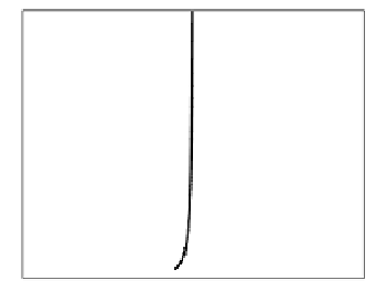
Fig. 5.1
f
E
(
e
)
for the continuous data splitter
tanh(
x−w
0
)
in a two-class Gaussian
problem with
μ
1
=
−μ
−
1
=2
and
σ
1
=
σ
−
1
=1
:a)
w
0
=
−
5
;b)
w
0
=
−
2
;c)
w
0
=0=
w
0
;d)
w
0
=5
.
error PDF is given by
f
E
(
e
)=
qf
E|−
1
(
e
)+
pf
E|
1
(
e
)
,
(5.7)
with (see Sect. 3.3.2.1)
exp
2
2
atanh
(
t−e
)
−
(
μ
t
−w
0
)
1
−
σ
t
√
2
πσ
t
e
(2
t
f
E|t
(
e
)=
1
,t
+1[
(
e
)
.
(5.8)
]
t
−
−
e
)
We note that
f
E
(0) is not defined but lim
e→
0
f
E
(
e
) exists and is zero. We now
analyze what happens when
w
0
varies. Figure 5.1 shows
f
E
(
e
) for different
values of
w
0
and the following settings of the two-class problem:
μ
1
=
−
μ
−
1
=
2 and
σ
1
=
σ
−
1
=1.For
w
0
→−∞
(of which Fig. 5.1a is an example),
f
E|−
1
and
f
E|
1
converge to Dirac-
δ
centered at
e
=
−
2 and
e
=0, respectively. A
similar behavior is found for
w
0
→
∞
where
f
E|−
1
and
f
E|
1
converge to a
+