Information Technology Reference
In-Depth Information
necessary to seize the nature of
δ
(
x
) because the origin is contained in the
nodes for
N
odd.
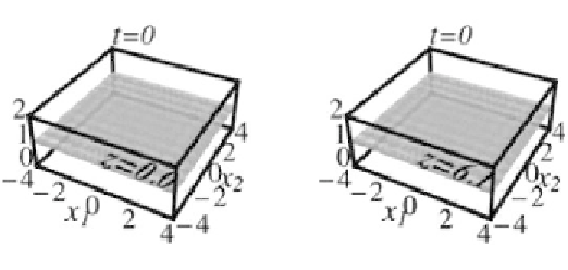
3.3.2 A UNIFORM DISTRIBUTION
We now take
u
(
x, t
) = 1 for
. Therefore, the solution of the inverse
problem (1) is
u
(
x
, 0) = 1. In other words, an initial uniform distribution of
temperature will be maintained the same at any future time. The numeri-
cal solution of the inverse problem (1) for this case, obtained by Eq. (9)
at the time
t
= 1,000 s, is given in Figure (
3.3). We display the numerical
results only on the
x
3
-planes:
x
3
= 0.0 and
x
3
= 6.1. For the displayed data
x
∈
3
on Figure (3.3), we have
E
0.0
=
E
6.1
= 10
−11
. Here,
x
3
= 6.1 corresponds
to the boundary upper
z
-plane.
FIGURE 3.3
Numerical approximation of
u
(
x
1
, x
2
, z,
0)= 1 for
z
= 0.0 and
z
= 6.1 obtained
by Eq. (9) with the final function
u
(
x, t
) = 1 at
t
= 1,000 s with
N
= 33. The values of the
approximated values
u
q
(0) are given on the vertical axis. The error for this case is 10
−11
.
3.3.3 A RADIAL DISTRIBUTION
As a third example, consider the distribution
2
2
2
xxx
+++
6 14)
α
t
+
α
t
()
222
123
1
2
3
−++
(
xxx
)/(1
+
4
α
t
)
uxt
,
=
e
,
(13)
(1
+
4
α
t
)
7/2
which has the solution
(
)
(
)
222
123
2
2
2
−++
(
xxx
)
ux
,0
=++
xxx
(14)
1
2
3


Search WWH ::

Custom Search