Graphics Reference
In-Depth Information
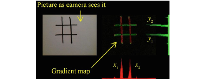
Fig. 8.2
Segmentation in action
1. Sum all of the gradients in the
x
-direction and find the two maximum values.
The two greatest horizontal gradient sums indicate where the horizontal lines are
located and we label these locations
y
1
and
y
2
. To find these two maximum gra-
dient sums, we use non-maximum suppression: after finding the first maximum,
we zero out the values next to the first maximum. This allows us to accurately
find the second peak, corresponding to the second horizontal line. By zeroing out
the pixels around the first maximum, we can prevent the issue of accidentally
mistaking a double peak as the second line.
2. Similarly, sum up all the gradients in the vertical-direction to obtain the two
maximum vertical sums (again using non-maximum suppression) so that, we
know the location of the vertical lines. We name the lines
x
1
and
x
2
.
3. Finally, we find the intersections of the four lines and can now access the contents
of the board cells.
Cell locations
. Once we determine the location of the four lines, we can use their
intersection points to find the nine cells. We first look at the central cell, with
x
1
,
x
2
,
y
1
, and
y
2
as its four bounding lines. We then find the rest of the tic-tac-toe cells
around the central cell.
“Empty” versus “full” detection
. Before we determine if a cell contains an X or
an O, we have to determine if it is empty or full. To that goal, we average the gradients
in each cell separately. If the gradient average is greater than an experimentally
determined threshold, the boxmust be full. If not, it is empty.We use gradients instead
of luminance in order to improve the robustness to global illumination changes.
If luminance was used for this purpose, the threshold would have to change as
illumination changes (Fig.
8.3
).
“X” versus “O” detection
. Once we determine that a cell is full, we need to know
which symbol is inside it.We do this by determiningwhere its centroid is (represented
by a blue dot on the display). Then, after we find the centroid, we consider a small box
around it, and average the gradients inside that box. The centroid, naturally, appears
close to the center of the shape, whether the box contains an X or an O, because both