Geography Reference
In-Depth Information
The cameras were controlled remotely using the camera
controller software available from Pine Tree Comput-
ing LLC and captured simultaneous time-lapse images
at intervals of 30-120 seconds during all of the high
flows as well as once at the beginning and end of each low
flow. Images were post-processed to correct for distortion
associated with lens curvature and perspective using the
Photoshop Andromeda Lensdoc plug-in. Each set of four
simultaneous images was stitched using the commercial
software PTGUI to create a single image.
Dye was added to the flow to enhance visualisation as
well as to measure flow depth based on colour-intensity.
Dyed water was made in batches by mixing 800 litres of
water in a large tank with Rhodamine dye at a concen-
tration of 2 ppm. The tank provided the only source of
water during the floods in order to maintain a constant
concentration of dye. Flow was recirculated with a pump.
This procedure was used for all experiments that had a
one-hour flood duration. In experiment with a four-hour
high flow photodegradation of the dye did not permit
flow recirculation. Instead, dye and water were fed in at
a constant rate at the inlet. Tilted trays with sand glued
to the bottom and sides were filled with dye water and
used to calibrate depth variation with colour intensity
(Figure 13.11). The calibration trays were placed at least
once during each flood in the field of view of each of the
four cameras and left permanently on the bed wherever
possible without disturbing the flow dynamics. The min-
imum calibration error associated with the calibration
trays was, on average,
Wetted widths and channel migration rates were
measured from flow maps created from time-lapse
images captured at 5 minute intervals during the floods.
Colour images were first converted into binary images in
which all the flow had a value of 1 (white) and all dry
areas (sand
+
veg) had a value of 0 (black; Figure 13.12a
and 13.12b). A threshold hue value of 0.8 and a saturation
value of 0.3 were used to distinguish between wet and
dry and the process was automated using Matlab. Data
were extracted along transects normal to the images and
spaced 0.05 m apart over the entire study reach (total of
226 transects). A cross-stream width of 0.06 m was set
as a threshold for a group of wet pixels to be considered
a channel. Wetted widths were calculated as the sum of
wet pixels averaged over a downstream distance of 0.3 m
(6 transects). Channel migration rates were calculated
by summing the area (in pixels) that was converted
from dry to wet between consecutive pairs of images
and dividing this area by the total length of the image.
Changes over 5-min intervals encompassed both gradual
lateral migration as well as abrupt (
<
5 min) channel
shifts from one location to another.
Analysis of flow maps for these experiments were used
to measure how wetted width, number of active channels
(braiding index), migration rates, and channel sinuosity
evolved as the braided channels transitioned to single-
thread channels (Tal and Paola, 2010). Similar to the
analysis described above by Kim and Paola (2007) and
using a technique developed by Wickert (2007), flow
maps were used to measure the timescale for loss of
pattern information, i.e. the time required for the entire
bed to get reworked once by the flow. The number of
pixels representing flow in the first image of a series that
1 mm. In order to minimise
calibration errors depth was estimated for each camera
separately using the tray for that image only, and as close
in time as possible to the time the image was captured.
+
/
−
6
4
2
0
0
50
100 150
Color value
200
250
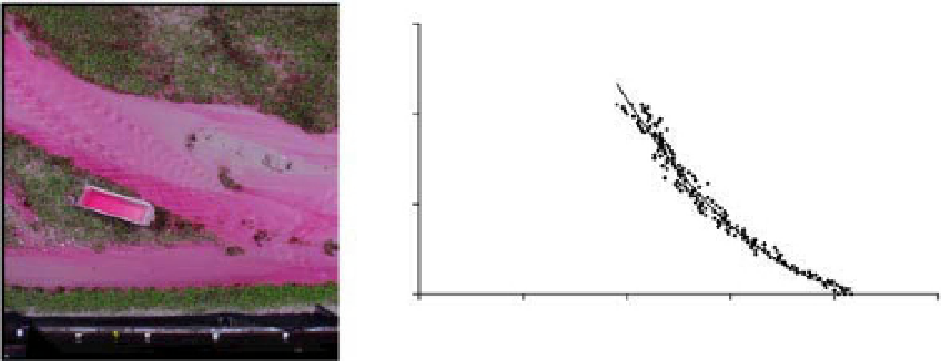
Figure 13.11
Flow with Rhodamine dye, calibration tray, and curve showing depth variation with colour intensity (Tal and Paola,
2007; Tal and Paola, 2010).
Search WWH ::

Custom Search