Geography Reference
In-Depth Information
This therefore assumes that the optical properties of the
shaded area are only modified by the presence of shad-
ing and that no physical properties of the river in terms
of bottom reflectance, depth or turbidity have changed.
Such spatial autocorrelation in river properties can be
reasonably assumed over short distances but disconti-
nuities may exist such as random boulders, man-made
bank stabilisation and localised incisions. We could easily
conceive of a case where the shaded area covers a pool at
the outside of a meander bend while the unshaded area
is limited to shallow water. In such a case, the algorithm
would use a shallow water histogram to correct a shaded
pool histogram and the results would inevitably be poor.
However, despite these 'what if?' considerations, in the
case of the Dartmouth river images used in Figure 8.11,
the assumption held and the results are promising. It
should be remembered that in the absence of any correc-
tions, the depth estimates in shaded areas have very large
errors. Therefore any correction method, even if imper-
fect represents an improvement. However, it should be
remembered that the image in Figure 8.11 is relatively
small and the channel change within each footprint was
generally small. In cases where channel change can be
important within a single image footprint, the assump-
tion that the unshaded area is a good approximation for
the shaded area may not hold and it could become nec-
essary to select unshaded pixels only in close proximity
to shaded areas in order to establish target histograms.
However, the ultimate, fundamental, limitation of this
method lies with the radiometric resolution of the sensor
and the compression of the histogram into few radio-
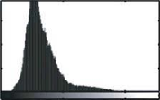
metric values. Figure 8.12 explicitly examines the effect
of shadows on the image histogram for the red band. In
Figure 8.12a, if we examine the histogram in the shaded
area, the width of this histogram at
1 standard deviation
is 4.6 DN. In the illuminated areas (Figure 8.12b), the
width is 27.8 DN. This demonstrates that the effect of
shading compresses the histogram to the point where a
very limited range of DN values are available. In such con-
ditions, the digitisation of the analogue emitted radiation
into a very limited number of integer DN values leads
to a significant loss of information. The only potential
improvement here is to improve the radiometric reso-
lution of the sensor (see Chapter 1 for a definition of
radiometric resolution). Unfortunately, this goes against
the current trend in river remote sensing instrumenta-
tion. Current commercial development efforts all seem
very focused on improving sensor resolutions and there
seems to be little impetus in the mainstream imaging
industry to produce high radiometric resolution cameras
on a mass scale thus lowering the cost of these devices.
This suggests that fluvial remote sensing is approaching
the point where customised, fit-for-purpose, instrumen-
tation will become a crucial step if substantive scientific
progress is to be maintained.
±
8.3.4 Imageclassification
Image classification is arguably the most fundamental of
all remote sensing analysis methods. This basic process
whereby the features in an image are first segmented into
distinct groups and then classified into a land-use type
(e.g. river, exposed bar and vegetation) is generally the
first step in any analysis of remotely sensed data. The
basic algorithms for this process all rely on the statistical
distribution of pixel brightness values in the available
bands in order to segment the image into groups of pixels
having similar spectral characteristics (Lillesand et al.,
3000
2000
2000
1000
1000
0
0
0
100
200
0
100
200
Image DN values
Image DN values
Shadow histogram
(a)
Bright histogram
(b)
Figure 8.12
Effects of shading on the image histogram. a) Shaded area histogram, b) Bright, unshaded, histogram for a
morphologically similar area.

Search WWH ::

Custom Search