Geography Reference
In-Depth Information
as a potential solution for shadow removal. However,
instead of referring to a reference image, we propose
the use of adjacent un-shaded areas in order to establish
normalisation targets. Conceptually this approach is very
similar to the normalised procedure described above.
First, image classification is used to delineate shaded and
non-shaded areas. Second, pixel histograms are extracted
for shaded and un-shaded portions of the river bed and
third, histogram equalisation is used to transform the
shaded area into a simulated unshaded area.
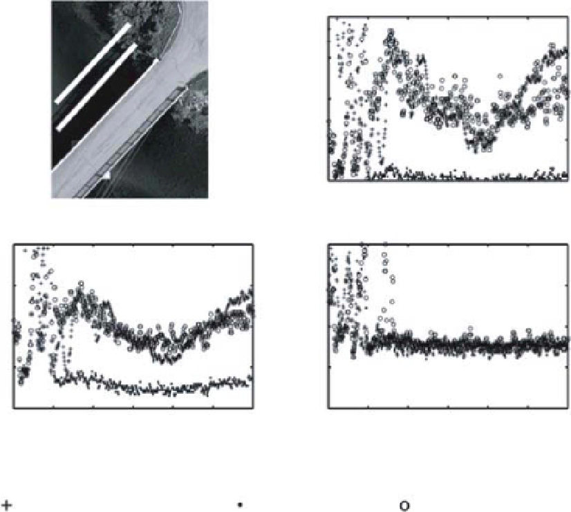
Figure 8.11 shows an example from the Dartmouth
River in Quebec, Canada. In this example, we have cho-
sen an image where a bridge spans the river and casts
a shadow across the entire channel width. The shadow
removal procedure discussed above will be used to resti-
tute the brightness values in the shaded area. In order to
assess the success of the procedure, we have defined two
cross sections A and B. Cross section A is immediately
outside the shaded area and cross section B is 3 meters
downstream of cross section A but well within the shaded
area. Given the close proximity of the two cross sections,
we would expect that their brightness profiles will be
very similar in unshaded conditions. In Figure 8.11,
we can see that prior to shadow removal, the shaded
and unshaded cross sections have significantly different
brightness values. The exception is the blue band where
shading seems to have had very little effect. However,
once shadow removal was performed, the corrected cross
section displays a cross sectional profile which becomes
very similar to the unshaded profile. This is a promis-
ing result which indicates that these targeted histogram
matching approaches have the potential of removing
shadows and of restituting channel bathymetry within
these areas.
However, the main conceptual problem with this
approach is the underlying assumption that the image
histogram for the bright, unshaded areas is a good
estimate of required histogram in the corrected areas.
100
RED
A
80
B
60
40
20
0
100
200
300
pixel
400
500
600
(a)
(c)
100
100
BLUE
GREEN
80
80
60
60
40
40
20
0
20
0
100
200
300
pixel
400
500
600
100
200
300
pixel
400
500
600
(b)
(d)
Profile A, unshaded
Profile B, raw
Profile B, corrected
Figure 8.11
Shadow correction procedure. a) Image where a bridge creates a shadow spanning the full channel. Effect of the
correction procedure (b) on the red band, (c) on the green band, and (d) on the blue band.
Search WWH ::

Custom Search