Environmental Engineering Reference
In-Depth Information
and 10-m
Q
a
derived from SSM/I using Chou et al. (
1995
,
1997
) technique which is
adjusted to the height of 2 m based on COARE 3.0 algorithm. All bulk variables are
also from NCEP/NCAR, NCEP/DOE, and ERA-40. The optimal fields of such
variables obtained by an advanced objective analysis approach (Yu and Weller
2007
) are then employed to compute LHF and SHF using COARE 3.0 algorithm.
One-degree daily mean (1985 onward) and monthly mean (1958 onward) data are
available at their website (
http://oaflux.whoi.edu/
).
11.5 Error Estimates and Uncertainties
Figures
11.1
,
11.2
, and
11.3
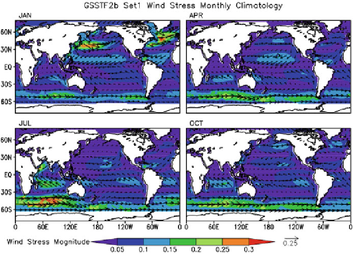
show examples of the seasonal variations of the stress,
sensible heat, and latent heat flux estimates. These seasonal climatologies are
computed from GSSTF2b set 1. Comparisons of the climatology, nonseasonal
variations, and trends of HOAPS, J-OFURO, and GSSTF2 are described elsewhere
(Chiu et al.
2008
,
2012
).
Certainly there are biases and uncertainties in surface turbulent flux products. The
flux biases can be classified into sampling errors, errors in the input bulk variables, and
Fig. 11.1
Wind stress climatology for January, April, July, and October from GSSTF2b set 1
(1998-2008). Unit: N m
2
Search WWH ::

Custom Search