Information Technology Reference
In-Depth Information
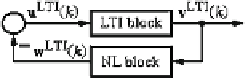
Fig. 8.5
Equivalent structure
of Eq. (
8.22
)
ε
=
ε
0
[
1
−
(
k
−
r
e
1
k
max
)/(
k
max
−
r
e
1
k
max
]
.
(8.24)
The input variable
i
v
is computed as the ratio of Popov sums
i
v
=
min
N
v
i
(
k
0
,
k
1
)/
max
N
v
i
(
k
0
,
k
1
)
∀
k
1
≥
k
0
≥
0
,
(8.25)
i
=
1
...
i
=
1
...
where the Popov sum is generally defined in the sufficient stability condition
k
=
k
0
(
k
1
w
LTI
i
T
v
LTI
i
2
0
v
i
(
k
0
,
k
1
)
=
(
k
))
(
k
)
≥−
μ
∀
k
1
≥
k
0
≥
0
,μ
0
=
const
,μ
0
=
0
,
a
i
(
a
i
(
w
LTI
i
a
i
(
a
i
(
T
(
k
)
=−[
k
)...
k
)
k
)...
k
)
]
,
q
i
x
q
i
v
LTI
i
1
i
x
i
T
=[
v
... v
...
]
,
(8.26)
resulted from the organization of Eq. (
8.22
) in terms of the equivalent structure given
in Fig.
8.5
and operating in the iteration domain.
The LTI block with dynamics in Fig.
8.5
is modeled by the state-space system
x
LTI
i
A
LTI
i
x
LTI
i
B
LTI
i
u
LTI
i
(
k
+
1
)
=
(
k
)
+
(
k
),
(8.27)
v
LTI
i
C
LTI
i
x
LTI
i
J
LTI
i
u
LTI
i
(
k
)
=
(
k
)
+
(
k
),
where
a
q
i
a
q
i
u
LTI
i
=[
a
i
a
i
a
i
a
i
T
...
...
]
,
q
i
x
i
x
LTI
i
v
LTI
i
1
i
2
i
x
i
x
i
T
=
=[
v
v
... v
...
]
,
ρ
i
diag
0
q
,
q
(
1
,
1
,...,
1
)
A
LTI
i
R
q
,
q
=
,
diag
(
1
,
1
,...,
1
)
∈
,
ρ
i
diag
(
1
,
1
,...,
1
)
diag
(
1
,
1
,...,
1
)
B
LTI
i
C
LTI
i
R
2
q
×
2
q
J
LTI
i
R
2
q
×
2
q
=
=
diag
(
1
,
1
,...,
1
)
∈
,
=
0
2
q
,
2
q
∈
.
(8.28)
The stability condition in Eq. (
8.26
) is derived from Popov's hyperstability con-
ditions (Precup et al.
2013a
). Equation (
8.26
) is a sufficient convergence condition
for GSA algorithms.
The complete rule bases of the two fuzzy logic blocks in the structure of the
second adaptive GSA are similar:
R
1
:
IF
i
v
IS N THEN
r
e
1
IS PS
,
R
2
:
IF
i
v
IS PS THEN
r
e
1
IS PB
,
(8.29)
R
3
:
IF
i
v
IS PB THEN
r
e
1
IS PS
,
Search WWH ::

Custom Search