Information Technology Reference
In-Depth Information
5
5
q=5.5 r=4.5
k
drag
= 7
q=5.5 r=4.5
k
drag
= 7
4
4
3
3
2
2
1
1
0
0
−1
−1
−2
−2
−3
−3
−4
−4
−5
−5
−10
−8
−6
−4
−2
0
−10
−8
−6
−4
−2
0
Real (s)
Real (s)
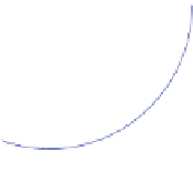
Fig. 6.5
Robot under fault occurrence: comparison between pole placement without FTC (
left
figure
) and pole placement with passive FTC (
right figure
)with
K
drag
=
7 kg/m
•
the reference is chosen as follows:
⎧
⎨
[0
.
1
,
0
.
2]
t
≤
15 s
x
ref
2
x
ref
4
[0
.
4
,
0
.
3]
15 s
<
t
≤
30 s
(
t
),
(
t
)
=
(6.33)
⎩
7]
T
[
−
0
.
3
,
−
0
.
30 s
<
t
≤
60 s
t
t
x
1
ref
x
2
ref
x
3
ref
x
4
ref
(
t
)
=
(τ )
d
τ
(
t
)
=
(τ )
d
τ
(6.34)
0
0
It can be seen that the controller has an intrinsic robustness against faults and
can tolerate them until a certain magnitude without loosing the system stability (e.g.
k
drag
=
5 kg/m, corresponding to the red line). However, taking a look at the position
of the poles under fault occurrence (Fig.
6.4
), it can be seen that even though the fault
k
f
5 kg/m does not affect the system stability, it compromises its performance,
as the desired specification in terms of poles location is no longer respected.
Using passive FTC, it is possible to enforce the robustness of the controller under
fault occurrence. Once a desired region of the complex plane has been chosen, it is
possible to find a lower bound for the faulty drag coefficient that makes the design
LMIs feasible. In this example, for the circle of center
drag
=
(
−
5
.
5
,
0
)
and radius 4
.
5, a limit
value of
k
drag
=
7 kg/m has been found. Figure
6.5
shows a comparison between the
closed-loop poles without FTC and the ones with passive FTC with such a value of
the faulty drag coefficient, for 10000 different realizations of the robot state matrix.
It can be seen that if no fault tolerance is enforced during the design phase, the poles
can escape from the desired region. The proposed approach avoids such undesired
behavior.


Search WWH ::

Custom Search