Computing a Model for Asset Management with Risk - Global Drinking Water Management and Conservation - page 181

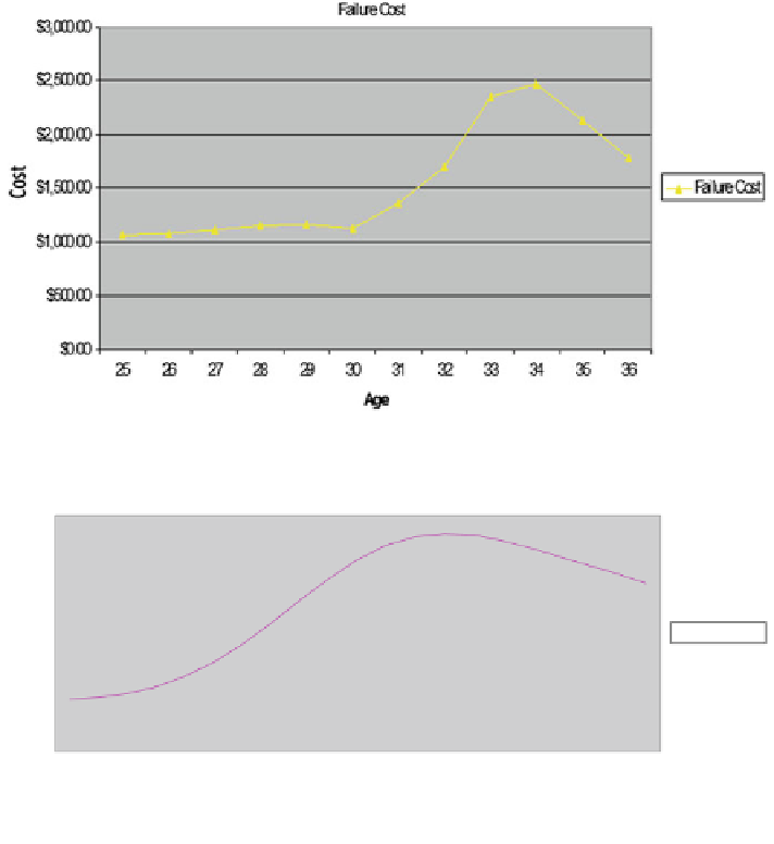
Fig. 8.12 S(x) in City B is nonlinear

Frequency

18

16

14

12

10

Frequency

8

6

4

2

0

16 17 18 19 20 21 22 23 24 25 26 27 28 29 30 31 32 33 34 35 36

Age

Fig. 8.13 F(x) in City B is nonlinear

e 0 : 0423x dx þ 119178e 0 : 0423t

t 1

R

22500e 0 : 22x
2250 þ 10 e 0 : 22x

0 : 25e 0 : 32x
25 þ 0 : 01 e 0 : 32x ð 1 Þ ð 1 Þ

1

C ðÞ¼ ð 8 : 17 Þ

1 e 0 : 0423 t þ 1

ð Þ

Continuous optimization of Eq. 8.17 yields a solution of 24.39. This solution is
con rmed by iterative graphical minimization as demonstrated in Figs. 8.16 and 8.17 .

8.4.4 City C

In City C, the same techniques as in Cities A and B were utilized. However, in this
city, the results were very different both in the linear and nonlinear analysis. The